Land surface temperature can be extracted from derived products, such as the MODIS Terra and Aqua satellite products (Wan 2006), or estimated directly from measurements in the thermal band. We will explore both options using the city of New Haven, Connecticut, USA, as the region of interest.
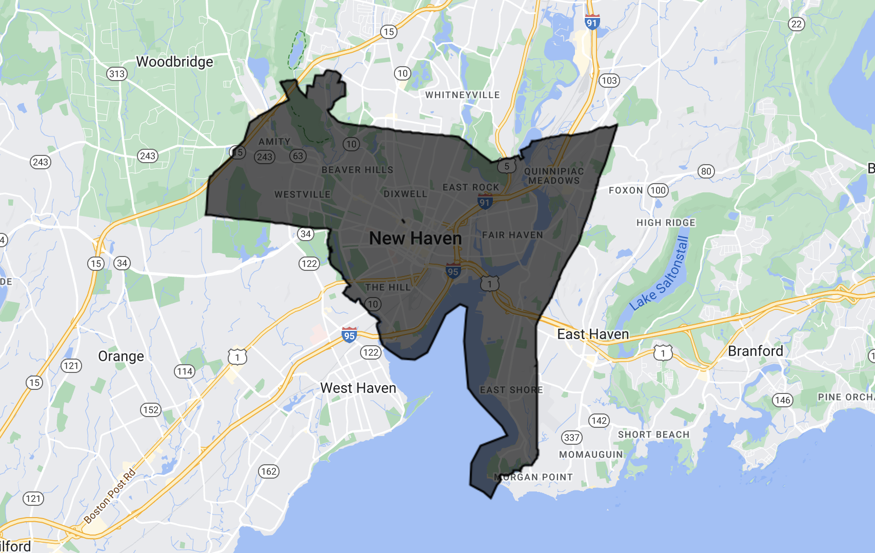
We start by loading the feature collection, which, being a census tract-level aggregation, we dissolve to get the overall boundary using the union operation. The FeatureCollection is added to the map for demonstration:
// Load feature collection of New Haven's census tracts from user assets.
var regionInt = ee.FeatureCollection("users/sounny/TC_NewHaven");

// Get dissolved feature collection using an error margin of 50 meters.
var regionInt = regionInt.union(50);

// Set map center and zoom level (Zoom level varies from 1 to 20).
Map.setCenter(-72.9, 41.3, 12);

// Add layer to map.
Map.addLayer(regionInt, {}, 'New Haven boundary');
Next we load in the MODIS MYD11A2 version 6 product, which provides eight-day composites of LST from the Aqua satellite. This corresponds to an equatorial crossing time of roughly 1:30 p.m. during daytime and 1:30 a.m. at night. In contrast, the MODIS sensor onboard the Terra platform (MOD11A2 version 6) has an overpass of roughly 10:30 a.m. and 10:30 p.m.
// Load MODIS image collection from the Earth Engine data catalog.
var modisLst = ee.ImageCollection('MODIS/006/MYD11A2');

// Select the band of interest (in this case: Daytime LST).
var landSurfTemperature = modisLst.select('LST_Day_1km');
We want to focus on only summertime SUHI, so we will create a five-year summer composite of LST using a day-of-year filter assembling images from June 1 (day 152) to August 31 (day 243) in each year:
// Create a summer filter.
var sumFilter = ee.Filter.dayOfYear(152, 243);

// Filter the date range of interest using a date filter.
var lstDateInt = landSurfTemperature
  .filterDate('2014-01-01', '2019-01-01')
  .filter(sumFilter);

// Take pixel-wise mean of all the images in the collection.
var lstMean = lstDateInt.mean();
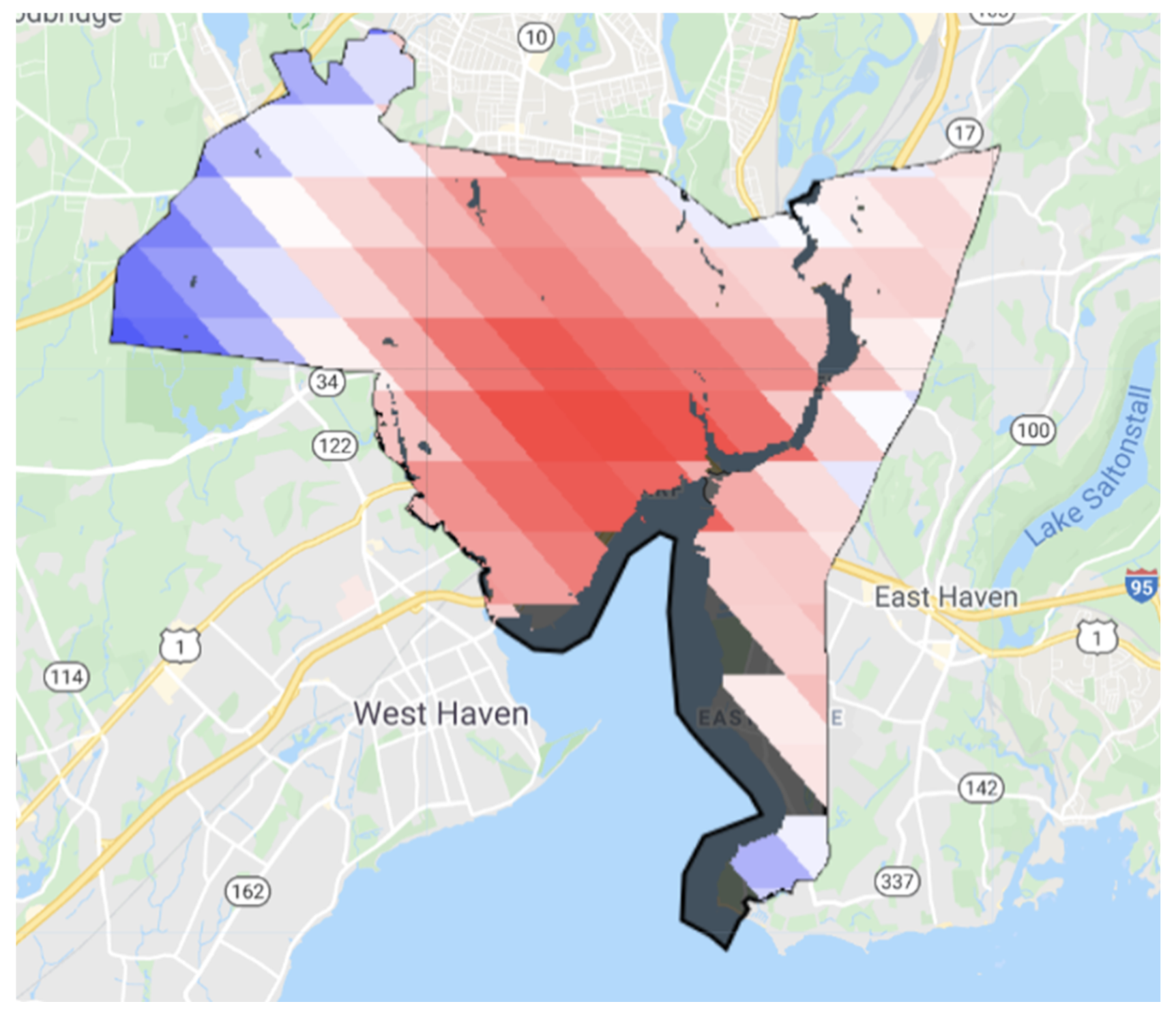
We now convert this image into LST in degrees Celsius and mask out all the water pixels (the high specific heat capacity of water would affect LST, and we are focused on land pixels). For the water mask, we use the Global Surface Water dataset (Pekel et al. 2016); to convert the pixel values, we use the scaling factor for the band from the data provider and then subtract by 273.15 to convert from Kelvin to degrees Celsius. The scaling factor can be found in the Earth Engine data summary metadata page.
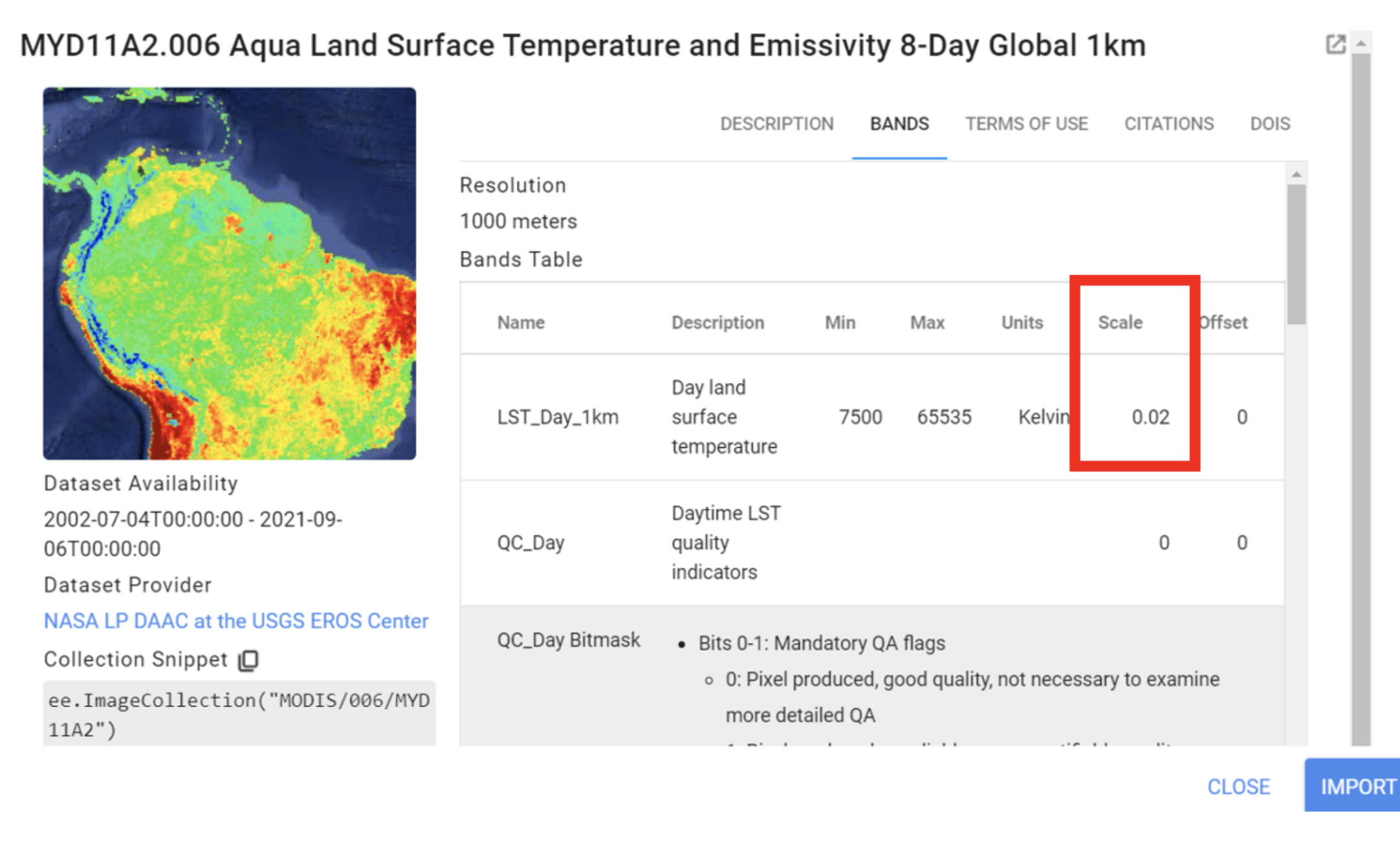
// Multiply each pixel by scaling factor to get the LST values.
var lstFinal = lstMean.multiply(0.02);

// Generate a water mask.
var water = ee.Image('JRC/GSW1_0/GlobalSurfaceWater').select('occurrence');
var notWater = water.mask().not();

// Clip data to region of interest, convert to degree Celsius, and mask water pixels.
var lstNewHaven = lstFinal.clip(regionInt).subtract(273.15)
  .updateMask(notWater);

// Add layer to map.
Map.addLayer(lstNewHaven, {
    palette: ['blue', 'white', 'red'],
    min: 25,
    max: 38
  },
  'LST_MODIS');