Workflow Integration Schedule
Foundations of Signal Integrity
Radiometric/Geometric Correction & Spectral Enhancement. Calibrating DNs into physical units and optimizing the 0-255 brightness range.
Break & Transition
Long Lunch & Data Ingestion for Afternoon Sessions. Prepare datasets for Change Detection & ML analysis.
Thematic Synthesis
Supervised/Unsupervised Classification and the Binary Hierarchical Classifier (BHC) Framework.
Temporal Dynamics
Change Detection, Phenology, and Ensemble Machine Learning for multi-temporal analysis.
Applied Excellence & Visualization
Random Forest Theory & Professional Cartographic Output. Publication-quality map composition.
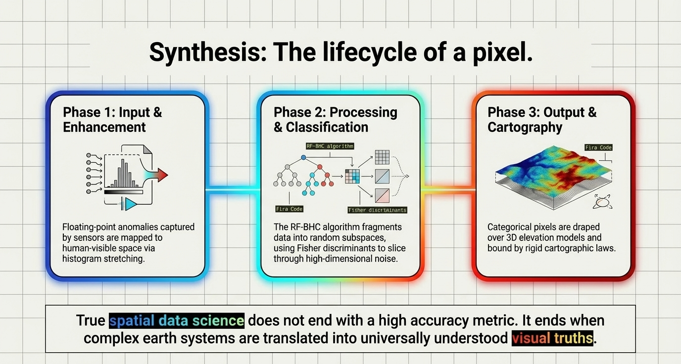
The Data Science Lifecycle: The progression from morning "Processing & Classification" to afternoon "Change Detection & AI" mirrors the actual professional lifecycle of geospatial data. We do not apply an ensemble classifier like Random Forest to raw data; we apply it to refined, spectrally consistent products. Refining the raw signal is the non-negotiable first step.
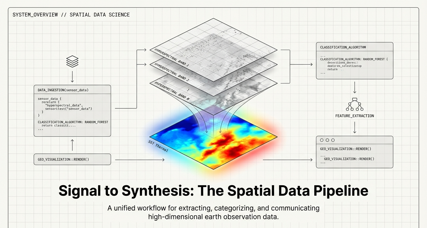
The Standard Processing Pipeline
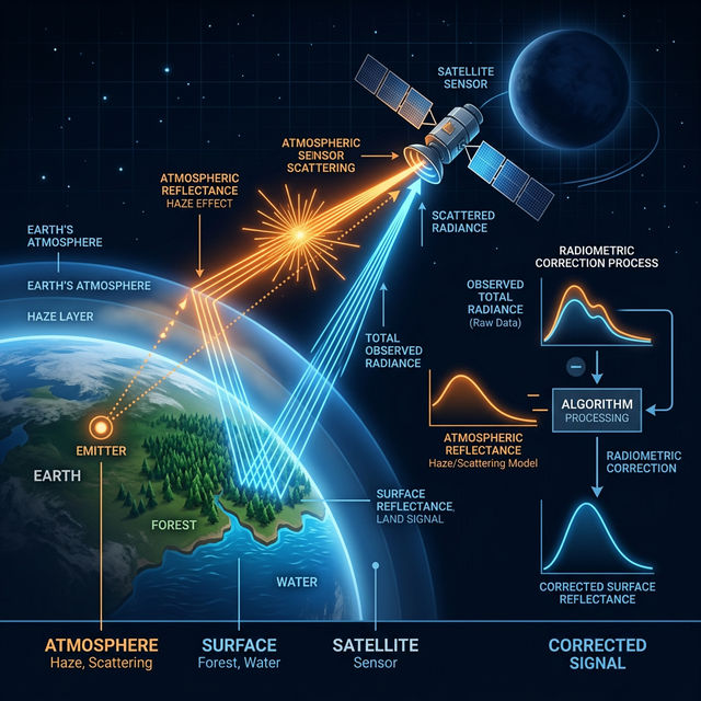
Raw satellite imagery is rarely suitable for immediate quantitative analysis. Atmospheric scattering and geometric distortions introduce errors that can invalidate downstream models. We must strategically remove these artifacts to ensure data integrity, particularly when dealing with floating-point data such as Sea Surface Temperature (SST) in the SEcoast.dat dataset or high-resolution Landsat TM scenes of Boulder, Colorado.
Morning Session Workflows
🔧 Radiometric Correction
Calibrating raw DNs into physical units (reflectance or degrees Celsius). Removes atmospheric haze and sensor noise.
📐 Geometric Correction
Aligning the image to a map coordinate system (UTM) so every pixel has a real-world location and scale.
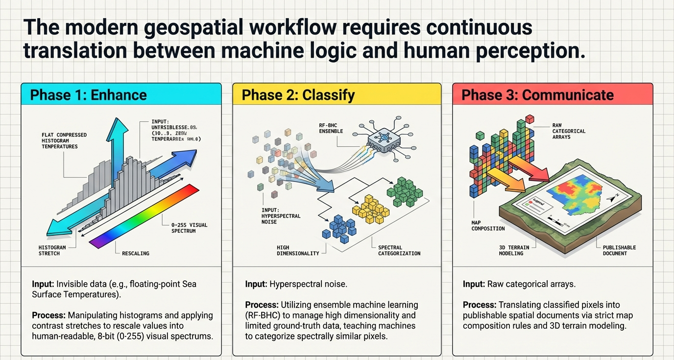
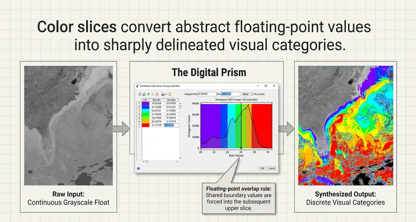
🎨 Image Enhancement
Rescaling data to optimize the 0-255 brightness range of digital displays for human interpretation.
🌿 Spectral Unmixing
A single pixel (e.g., 250m MODIS) is a mix of signatures. Just as Purple is a product of red and blue light, a pixel may contain grass, soil, and water. Unmixing "unpacks" the signal to find the proportional reality beneath.
graph LR
    A["Raw Data (DN)"] --> B["Radiometric Calibration"]
    B --> C["Atmospheric Correction"]
    C --> D["Surface Reflectance"]
    D --> E["Feature Engineering"]
    E --> F["ML Classifier"]
    F --> G["Thematic Map"]
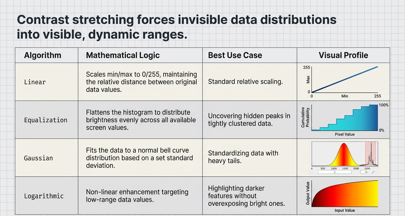
Strategic Application of Contrast Stretches
Contrast stretching rescales input data (often floating-point or 16-bit) into the 8-bit (0-255) integer range required for visualization. Each method has a unique strategic application:
| Stretch Type | Mechanism | Strategic Application |
|---|---|---|
| Linear (1/2/5%) | Clips a specified % of histogram tails and stretches the remainder | Standard for general visualization; avoids outliers like clouds |
| Equalization | Scales the input distribution to use the full 0-255 range equally | Best for highlighting subtle variations in high-density data regions |
| Gaussian | Fits data to a normal distribution based on standard deviation | Enhances features in the middle of the spectral distribution |
| Square Root | Takes the square root of the input histogram before linear stretch | Compresses highs to reveal details in darker shadow regions |
| Logarithmic | Non-linear enhancement of low-range brightness values | Essential for dark features or low-reflectance targets |
| Optimized Linear | Dynamic range adjustment optimized for 16-bit integer data | Maximizes information in midtones, highlights, and shadows |
"So What?" Layer: Statistical Feature Isolation. The distinction between "Stretch on View Extent" and "Full Extent" is a critical laboratory skill. In the SEcoast.dat image, a significant area of negative values near the bottom can skew global statistics, washing out terrestrial features. By utilizing "Stretch on View Extent," we recalculate statistics based only on visible pixels, effectively isolating land features from the high-variance ocean background.
Classification Frameworks
The transition from spectral signatures to thematic knowledge requires a choice between Unsupervised (ISODATA/K-means) and Supervised classification. This choice is governed by the availability of "ground truth" (high-quality labeled training data) and the required degree of human intervention.
Challenges in Hyperspectral Classification
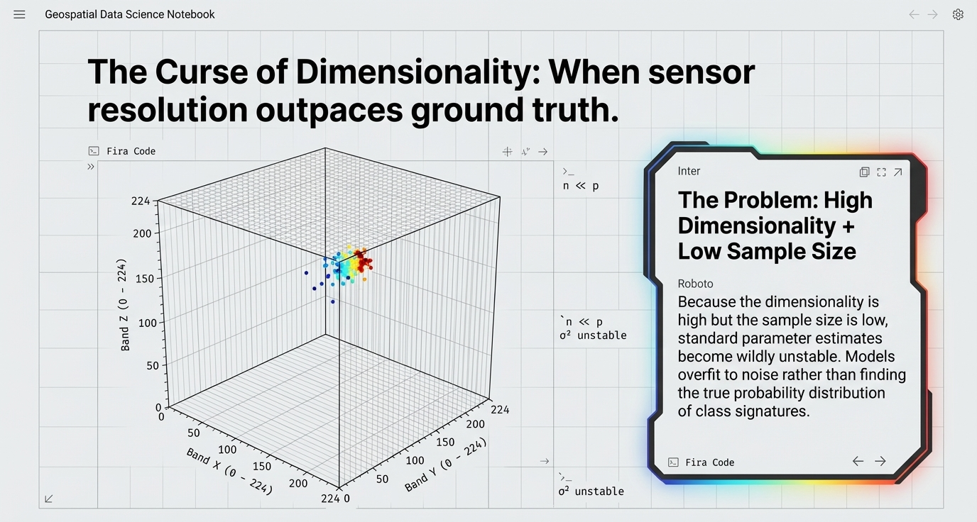
Statistical classification of hyperspectral data is complex due to high dimensionality and limited ground truth.
- Dimensionality & Sample Size: High-dimensional data requires massive training sets. Small training sets cause standard parameter estimates to become unstable.
- The Hughes Phenomenon: As dimensionality increases, if the sample size is low, the model overfits to noise rather than finding the true probability distribution.
🤖 Unsupervised Classification
Algorithms cluster pixels based on inherent spectral similarities without prior "ground truth". The "Big Two" are:
- K-Means: Fast and simple. You specify a fixed number of clusters, and it assigns pixels based on simple spectral distance.
- ISODATA: Iterative Self-Organizing Data Analysis Technique. A "smarter" algorithm where you specify a range of clusters; it dynamically splits clusters with high variance and merges clusters that are statistically similar.
Advanced Strategy (Pseudo-Labeling): Sometimes, unsupervised outputs are noisy. You can use K-Means clusters as "labels" to train a Random Forest, which "cleans up" the classification by finding generalized patterns.
🎯 Supervised Classification
Involves training an algorithm with expert-defined ground truth (ROIs). The Art of Training: Proximity matters. You cannot cluster all training points in one spot; you must spread samples across the spectral and spatial extent of the scene to capture variance. The reliability of the output is a direct function of the cleanliness and representativeness of your training data.
🧠 Human Agency vs. The Technological Ceiling
While supervised models learn from us, humans have a unique history of breaking "fixed" environmental rules:
- Beyond Malthusian Limits: Historically, theorists like Thomas Malthus attempted to calculate physical "ceilings" for population based on land. However, through the Green Revolution and intensive engineering (irrigation, genetic engineering), humans consistently overcome these environmental boundaries.
- The Policy Duality: In SpaceApps, we recognize that while RS can map a physical limit, human policy and ingenuity are what determine if that limit becomes a collapse or a transition.
The Cognitive Metaphor: Classification is the most natural human approach. Just as a baby sees the world and groups objects into "goes in mouth" or "doesn't go in mouth" long before learning the word "food," unsupervised algorithms find patterns first; we provide the labels (the words) later.
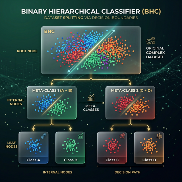
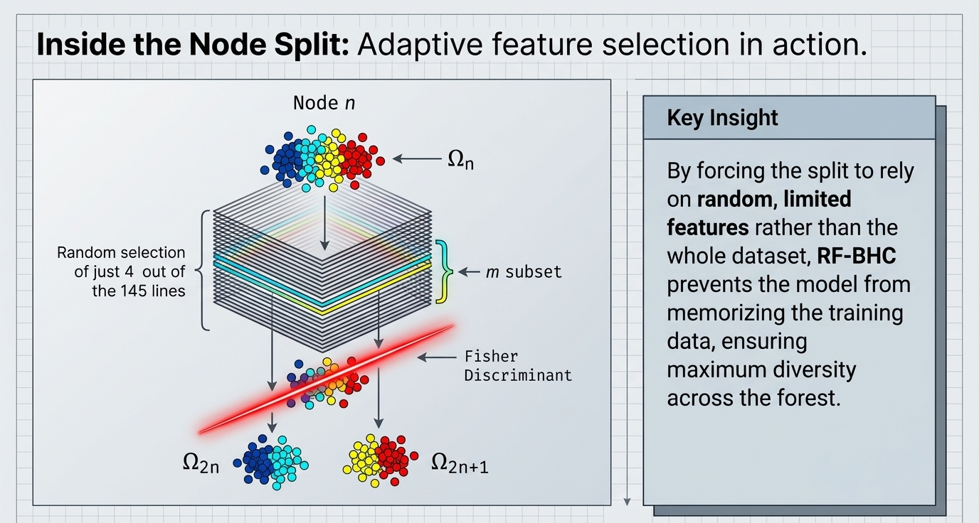
The Binary Hierarchical Classifier (BHC)
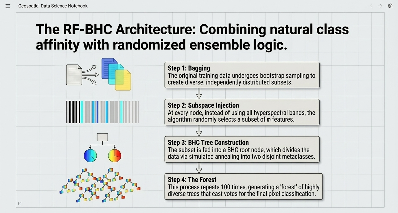
As detailed in the Ham et al. (2005) research, the BHC utilizes a "divide-and-conquer" logic to manage large output spaces in hyperspectral environments:
graph TD
    A["All Classes"] --> B{"BHC Root Split"}
    B -->|"Meta-Class A"| C["Water + Wetlands"]
    B -->|"Meta-Class B"| D["Land Covers"]
    C --> E{"Sub-Split"}
    E --> F["Open Water"]
    E --> G["Marsh / Swamp"]
    D --> H{"Sub-Split"}
    H --> I["Forest Types"]
    H --> J["Urban / Bare Soil"]
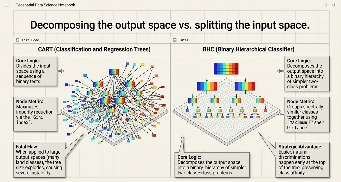
- Recursive Decomposition: Breaks a multi-class problem into a tree of simpler two-class (meta-class) problems.
- Class Affinity: The root classifier partitions classes based on natural spectral similarity, allowing easier discriminations (e.g., Water vs. Land) at the top of the hierarchy.
- Simulated Annealing: Employs the Generalized Framework for Associative Modular Learning Systems (GAMLS) to determine optimal splits.
"So What?" Layer: The Curse of Dimensionality. In hyperspectral environments like the Kennedy Space Center (NASA AVIRIS) or the Okavango Delta (Hyperion), when the number of spectral bands is high and training samples are small, traditional classifiers become unstable. Frameworks like BHC reduce this redundancy while maintaining discriminative power.
Change Detection & Temporal Dynamics
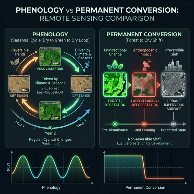
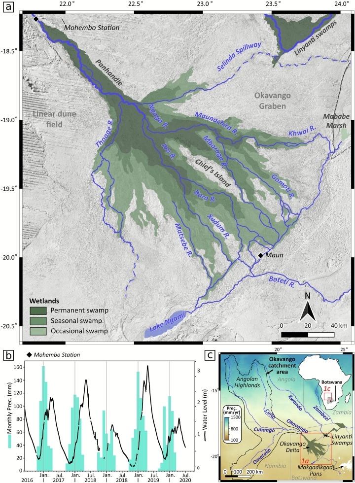
Temporal analysis allows us to distinguish between human-driven conversion and natural phenology. This is particularly salient in the distal portion of the Okavango Delta, where seasonal flooding (hydroperiods) dictates vegetation response.
Critical Distinction: Phenology vs. Conversion
🔄 Phenological Cycles (Seasonal)
Predictable variations in spectral response, such as "Hippo Grass" (Class 2) which is seasonally inundated. These represent fluctuating states of the same land cover type.
🔀 Permanent Conversion
A fundamental state shift, such as conversion of "Acacia Woodlands" into settlements. Represents an irreversible change.
Determinism vs. Governance: Jared Diamond's "Collapse" narrative argues that environmental shifts determine civilizational failure (e.g., Syria's drought). However, a critical distinction in Land Change Science and the study of Coupled Human-Natural Systems is required: while satellite imagery may confirm a drought, drawing a line to causation requires careful interpretation.
📊 RS Science & Policy: Multi-temporal Remote Sensing (e.g., NASA MODIS/Landsat) acts as the Common Operating Picture for policy-makers. By establishing an objective biophysical baseline, RS forces a debate on whether a crisis is a result of natural "triggers" or systemic "governance failure," moving policy from reactive relief to proactive institutional reform.
graph LR
    A["Time 1 Image"] --> C["Image Differencing"]
    B["Time 2 Image"] --> C
    C --> D{"Threshold Analysis"}
    D -->|"Within range"| E["No Change"]
    D -->|"Exceeds range"| F["Change Detected"]
    F --> G{"Temporal Pattern"}
    G -->|"Cyclic"| H["Phenology"]
    G -->|"Permanent"| I["Land Cover Conversion"]
Algebraic vs. Machine Learning Strategies
Monitoring environmental shifts requires robust statistical models over raw pixel subtraction.
- Algebraic Methods (Image Differencing): Employs a corner method to establish empirical change thresholds between multi-temporal images. Fast, but prone to error in complex scenes.
- Machine Learning (Post-Classification): Utilizes a decision tree induction algorithm and a post-classification separability matrix. Experimental evaluation on Landsat data proves this ML approach delivers superior accuracy for tracking human impacts and land cover permanent changes.
Okavango Case Study: The Okavango Delta's annual flood pulse creates a dynamic landscape. Using multi-temporal EVI composites (derived from EO-1 Hyperion), we can distinguish between vegetation zones that respond to seasonal inundation versus those that have permanently shifted due to hydrological or anthropogenic changes.
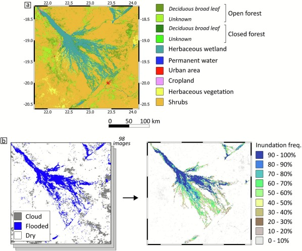
Source: ScienceDirect - Investigating spatial and temporal dynamics of the Okavango Delta
Advanced AI & ML: The Random Forest Framework
To understand a Random Forest, we must first understand its building block: CART (Classification and Regression Trees). A CART is a non-parametric decision tree that handles complex, non-linear satellite data by asking a series of "Yes/No" questions (e.g., "Is the Short-Wave Infrared value very low?"). Unlike older models, CART does not care if your data is "normally distributed."
However, a single CART is prone to Overfitting—it can memorize the noise in specific imagery rather than learning general landscape patterns. The Random Forest (RF) solves this by acting as a "committee of experts." By combining multiple decision trees, RF achieves stability that single-tree models cannot match.
The RF Mechanism
The framework enhances classification through several key mechanisms:
- Ensemble Voting: Hundreds of individual trees independently classify a pixel; the final output is the category selected by the majority block.
- Robustness to Noise (Bagging): Bootstrap Aggregating. Every tree is trained on a random subset of the data, ensuring no single anomaly dictates the outcome.
- Feature Randomness: At every node split, the algorithm randomly selects a subset of features (bands) rather than evaluating all of them. This ensures the trees are "de-correlated" and don't all make the identical mistakes.
- Handling Imperfect Data: Readily manages missing values via surrogate splits and excels with small or imbalanced ground-truth datasets.
- Feature Importance Assessment: Naturally calculates "variable importance," allowing analysts to rank which specific spectral bands are most critical for class separation.
graph TD
    S["Full Training Dataset"] --> B1["Bootstrap Sample 1"]
    S --> B2["Bootstrap Sample 2"]
    S --> Bn["Bootstrap Sample N"]
    B1 --> T1["🌲 Tree 1 - Random Subset of Bands"]
    B2 --> T2["🌲 Tree 2 - Random Subset of Bands"]
    Bn --> Tn["🌲 Tree N - Random Subset of Bands"]
    T1 --> V{"🗳️ Majority Vote"}
    T2 --> V
    Tn --> V
    V --> F["Final Classification Map"]
Comparative Analysis: RF-BHC vs. RF-CART
Based on research conducted at the University of Texas Center for Space Research:
| Method | Diversity (Entropy) | Accuracy (Small Samples) | CPU Time |
|---|---|---|---|
| RF-BHC | Lower (Class Affinity) | Higher; exploits spectral groupings | 1h 4m 4s (Simulated Annealing) |
| RF-CART | Higher (Diverse Trees) | Lower; depends on training statistics | 8m 42s (Standard CART) |
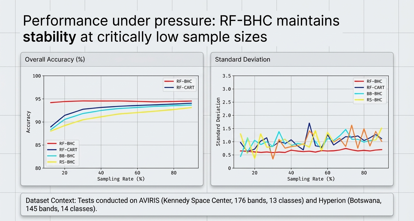
"So What?" Layer: Stability and Generalization. The "Majority Vote" is the secret to RF's success. By averaging many "weak" learners, the ensemble becomes robust against overfitting and outliers. This is especially effective for spatially disjoint areas where class-conditional feature distributions vary.

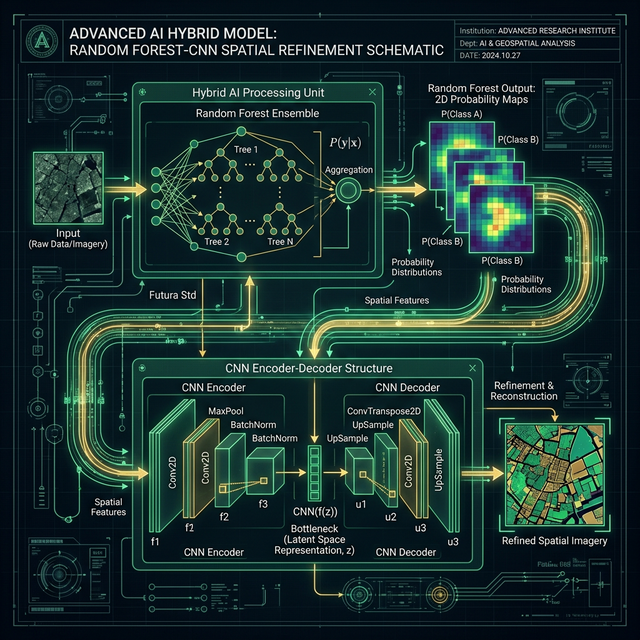
Advanced Hybrids: RF + Convolutional Neural Networks (CNN)
Traditional classifiers like Random Forest often treat a satellite image like a "bag of pixels", ignoring surrounding neighbors. CNNs (Convolutional Neural Networks) work like the human eye. They scan the image using "Convolution" to detect low-level features (edges), mid-level features (shapes), and high-level features (objects like a pivot irrigation field or ship). They are the gold standard for object detection and semantic segmentation.
CNN vs. CCN Clarity: In Geography, do not confuse CNN (a deep learning machine logic) with CCN (Cloud Condensation Nuclei). CCN are physical aerosols (dust, sea salt) crucial for atmospheric correction and climate modeling that provide the seed surface for water vapor condensation, leading to the Twomey Effect.
Modern spatial data science bridges RF simplicity and CNN spatial awareness using deep learning hybrids:
- Phase 1 (Pixel-Wise RF): RF handles noisy high-dimensional data, extracting spectral features to generate 2D probability maps identifying likely targets (e.g., distinguishing oil from water). Predictions may be spatially fragmented.
- Phase 2 (CNN Spatial Refinement): Instead of feeding massive raw 3D data into a CNN, the CNN takes the RF's 2D probability maps as inputs. Using an Encoder-Decoder architecture, the encoder max-pools to find broad context, and the decoder restores spatial resolution.
- The Result: The hybrid bridges pixel-level probabilistic logic with intelligent spatial feature learning, yielding perfectly contextualized boundaries.
Global Research Network & Applied Excellence
Remote Sensing is a collaborative endeavor integrating climate dynamics, social science, and GeoAI to solve sustainability challenges. Here are key individuals shaping the field:
Faculty Spotlight

Known for integrating remote sensing with social sciences. Her work highlights how human decisions and climate variability interact to drive landscape changes in vulnerable semi-arid regions.

A leading expert utilizing remote sensing to assess climate change impacts on global vegetation. Her research models how agricultural and natural landscapes respond to shifting climatic envelopes.

Focuses on big Earth data and cloud computing (Google Earth Engine) applied to global sustainability challenges, mapping high-resolution ecosystem dynamics using advanced ML.

Specializes in integrating drone imagery with satellite data for precision agriculture and forestry management, utilizing ML to bridge the gap between field and orbital scale.
ISU Research Highlights

Norbert is a data science professional developing intelligent space-enabled solutions. In his ISU research, he integrated systems engineering, AI, and GeoAI sensing to advance environmental resilience. He conducted a seminal 25-year EVI time series analysis (2000–2025) of the Okavango Megafan using Google Earth Engine, proving the flood-driven resilience of wetland cores versus climate-sensitive dryland margins.
Explore Megafans Research
Specialized in automated feature extraction within complex imagery environments. His graduate work and research proposals tackle spatial analysis challenges, mapping rapid environmental changes with AI.
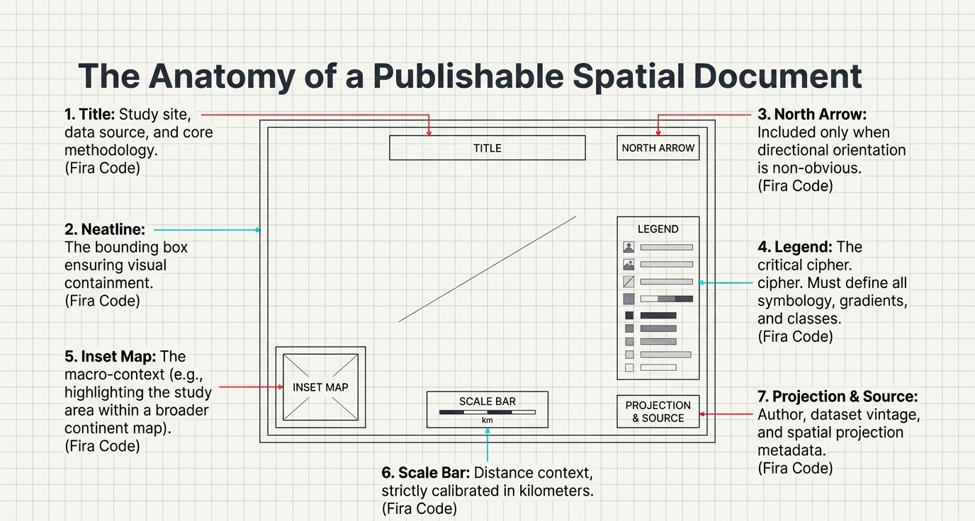
Professional Cartographic Communication
A sophisticated model is undermined by poor communication. Publishable maps must translate complex data into accessible knowledge for decision-makers.
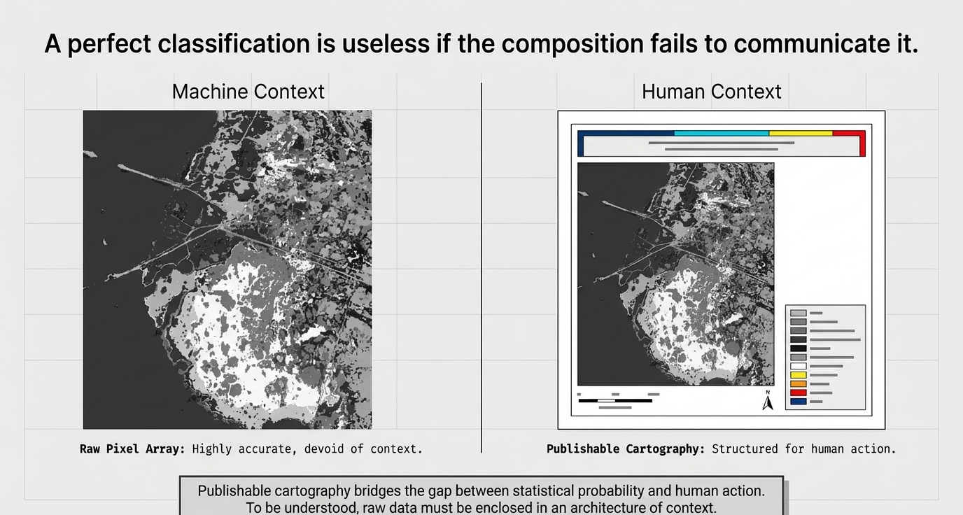
The Seven Essential Map Elements
Data, location, date
Clean map frame
Orientation reference
All symbology keys
Geographic context
Author, date, sensor
Always in Kilometers
Best Practices: 3D Surface Visualization
To model topographic complexity (e.g., the Boulder, CO dataset), we combine spectral imagery with a Digital Elevation Model (DEM).
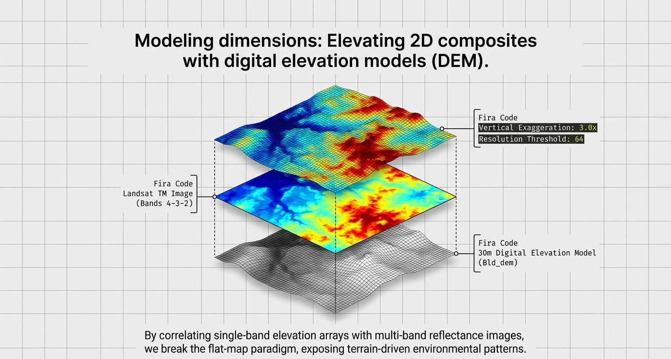
| Parameter | Recommended Value | Rationale |
|---|---|---|
| DEM Resolution | Full or 64 | Maximum topographic detail |
| Vertical Exaggeration | Factor of 3.0 | Multiplies elevation values by a defined factor to make topographic relief distinct and obvious. |
| Elevation Threshold | Min Plot Value: 1500m | Focus on relevant terrain features |
Checklist for Publishable Maps
- ☐ Ensure all units are in Kilometers.
- ☐ Apply Graticules (Lat/Long grids) for professional reference.
- ☐ Verify legible text annotations for major features (e.g., "Gulf Stream").
- ☐ Metadata Citation: Clearly cite data sources as "NASA AVIRIS" or "EO-1 Hyperion."
- ☐ Export final compositions as high-resolution TIFF or JPEG for publication.
Regional Decisions: The Cartographer's Dilemma
Scenario: You are mapping permanent land cover conversion in the Okavango for policymakers managing water rights. Your standard linear stretch makes seasonal swamps look identical to permanent urbanization due to overlapping spectral responses.
Decision: Do you present a raw classification table that is accurate but unreadable, or do you apply an aggressive Gaussian stretch and 3D terrain exaggeration that makes the map beautiful but potentially exaggerates the scale of water loss? How do you balance statistical integrity with compelling political communication?
🎓 Knowledge Check
Test your understanding of today's lecture material.
1. Why is it critical to perform radiometric correction BEFORE applying a Random Forest classifier?
2. What is the key advantage of the BHC framework over traditional multi-class classifiers for hyperspectral data?
3. How does Random Forest achieve stability against overfitting?
4. In change detection, what distinguishes a phenological cycle from permanent land cover conversion?
Summary of Big Ideas
- ✓ Signal Integrity is Non-Negotiable: Raw data must be corrected radiometrically and geometrically before any quantitative analysis. Garbage in, garbage out.
- ✓ Classification is a Spectrum: From simple K-means to sophisticated BHC hierarchies, the choice depends on data complexity and available ground truth.
- ✓ Temporal Context Matters: Distinguishing phenology from conversion prevents misclassification in dynamic environments like the Okavango Delta.
- ✓ Ensemble Methods Win: Random Forest's "majority vote" provides stability that single-tree classifiers cannot, especially with limited training data.
- ✓ Communication is Science: A publishable map with all seven essential elements is the final, critical step in the scientific workflow.