What You'll Learn
- Collect training data using the Geometry Tools in Earth Engine
- Configure FeatureCollections with class properties for training
- Train a CART (Classification and Regression Tree) classifier
- Train a Random Forest classifier and compare results
- Interpret classification results and identify sources of error
Building On Previous Learning
This lab builds on Lab 8 (band selection and indices) and the Classification Types module where you learned the theoretical differences between unsupervised and supervised classification.
Why This Matters
Supervised classification is the industry standard for creating accurate land cover maps. It's used for:
- Urban planning: Mapping impervious surfaces and green spaces
- Agriculture: Identifying crop types and estimating planted area
- Conservation: Monitoring habitat loss and ecosystem changes
- Climate research: Creating inputs for climate and hydrological models
Random Forest, which you'll learn in this lab, is one of the most widely-used classifiers in remote sensing research.
Before You Start
- Prerequisites: Complete Lab 10 and watch the supervised classification walkthrough in the module.
- Estimated time: 75 minutes
- Materials: Earth Engine login, training sample plan, and accuracy assessment worksheet from the lecture.
Key Terms
- Training Data
- Labeled samples where you know the true land cover class, used to teach the classifier.
- Feature Collection
- A collection of Features (geometries with properties) in Earth Engine, used to store training points.
- Class Property
- A numeric attribute assigned to each training sample indicating its land cover class (e.g., 0=Forest, 1=Urban).
- CART (Classification and Regression Tree)
- A decision tree algorithm that creates rules based on band values to classify pixels.
- Random Forest
- An ensemble classifier that builds many decision trees and uses voting to determine the final class.
- Hyperparameters
- Settings that control how a classifier learns (e.g., number of trees in Random Forest).
Introduction
Supervised classification uses a training dataset with known labels representing the spectral characteristics of each land cover class of interest to "supervise" the classification. The overall approach in Earth Engine follows these steps:
- Get a satellite scene
-
Part 1 - Load the Satellite Image
We will begin by loading a clear Landsat 8 image. We'll use a point in Milan, Italy, as the center of our study area.
// Create an Earth Engine Point object over Milan.
var pt = ee.Geometry.Point([9.453, 45.424]);

// Filter the Landsat 8 collection and select the least cloudy image.
var Landsat = ee.ImageCollection('LANDSAT/LC08/C02/T1_L2')
    .filterBounds(pt)
    .filterDate('2019-01-01', '2020-01-01')
    .sort('CLOUD_COVER')
    .first();

// Center the map on that image.
Map.centerObject(Landsat, 8);

// Add Landsat image to the map.
var visParams = {
    bands: ['SR_B4', 'SR_B3', 'SR_B2'],
    min: 7000,
    max: 12000
};
Map.addLayer(Landsat, visParams, 'Landsat 8 image');
Understanding the code:
.sort('CLOUD_COVER')- Orders images by cloud cover percentage.first()- Takes the least cloudy image (first after sorting)- The visParams display a true-color composite (Red-Green-Blue)
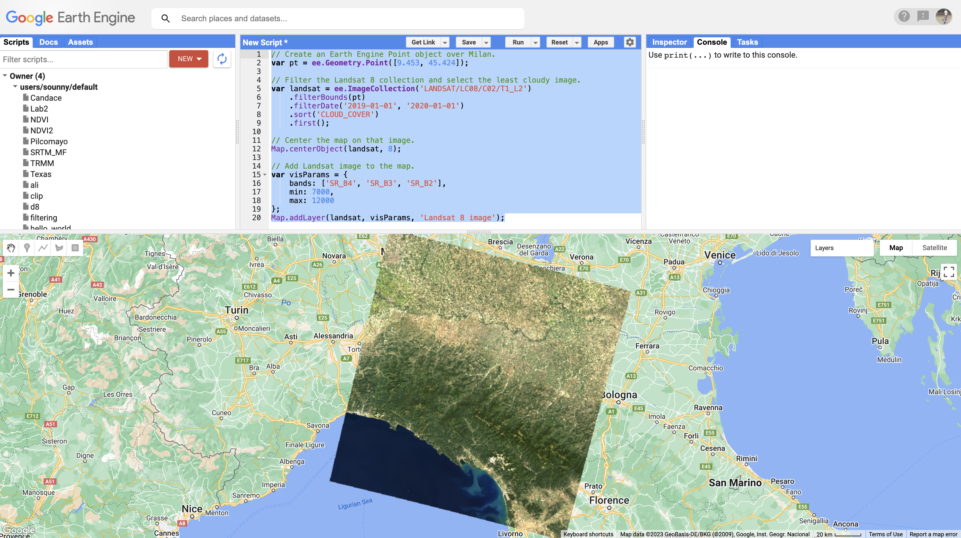
Landsat 8 true-color image of Milan, Italy -
Part 2 - Define Your Land Cover Classes
Before collecting training points, define the classes you want to map. For this exercise, we'll use four classes:
Class Name Class Code Hex Color Description Forest 0 #589400 Trees and dense vegetation Developed 1 #FF0000 Urban areas, buildings, roads Water 2 #1A11FF Rivers, lakes, sea Herbaceous 3 #D0741E Crops, grassland, bare fields Why numeric codes? Classifiers work with numbers, not text. The palette in your visualization will map these codes back to meaningful colors.
-
Part 3 - Collect Training Points
Now we'll use the Geometry Tools to create points on the Landsat image representing each land cover class.
Step 3a: Create the First Feature Collection
- In the Geometry Tools, click on the marker (point) option
- A geometry import named "geometry" will appear. Click the gear icon to configure it
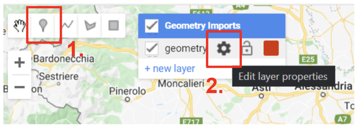
The Geometry Tools in the Code Editor Step 3b: Configure the Feature Collection
- Name the import
forest - Change the import type to FeatureCollection
- Click + Property
- Name the property
classand set its value to0 - Set the color to
#589400(dark green) - Click OK
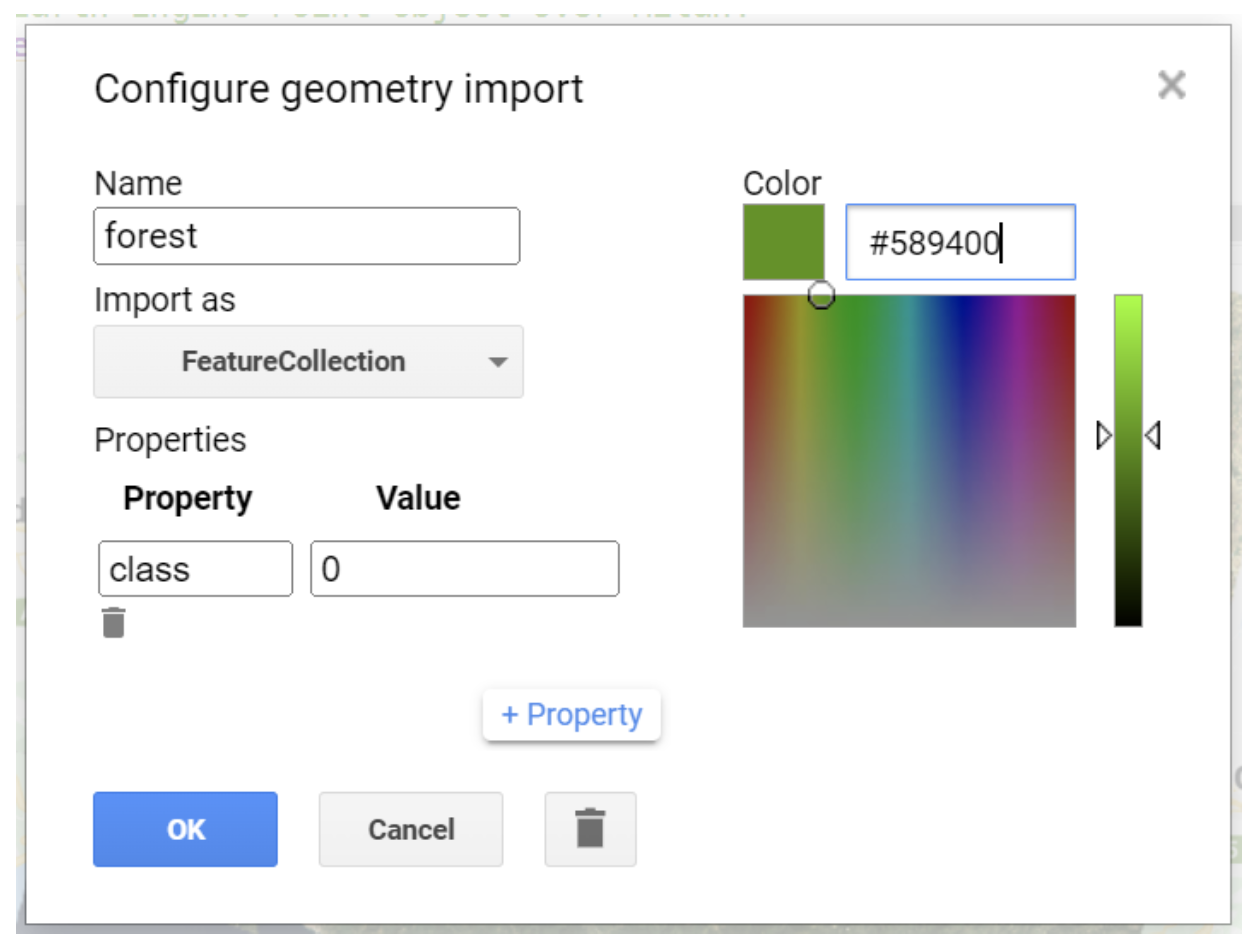
Configuring the forest FeatureCollection with class property About Hexadecimal Colors: Hex colors use six digits (0-9, A-F) in pairs for Red, Green, and Blue. For example,
#589400has 58 red, 94 green, and 00 blue - creating a dark green.#FF0000is pure red.Step 3c: Collect Forest Points
- Click on
forestin the Geometry Imports to activate drawing mode - Click on forested areas in your Landsat image
- Collect at least 25 points
- Click Exit when finished
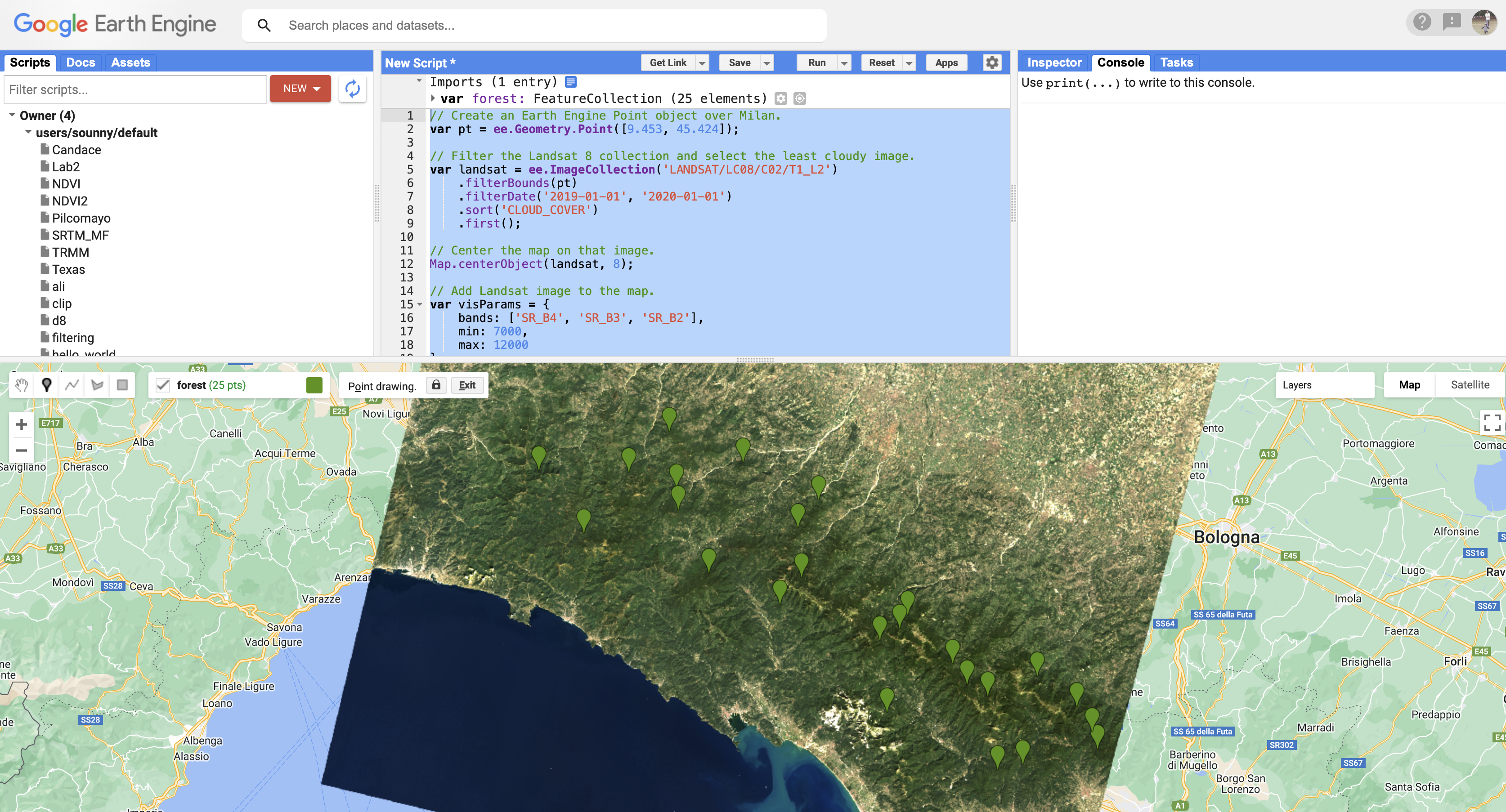
Forest training points collected across the study area Step 3d: Repeat for Other Classes
Create new layers for each remaining class. For each one:
- Developed: class = 1, color = #FF0000, collect over urban areas
- Water: class = 2, color = #1A11FF, collect over the sea and rivers
- Herbaceous: class = 3, color = #D0741E, collect over agricultural fields
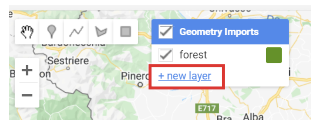
Click the "+ new layer" button to create each class 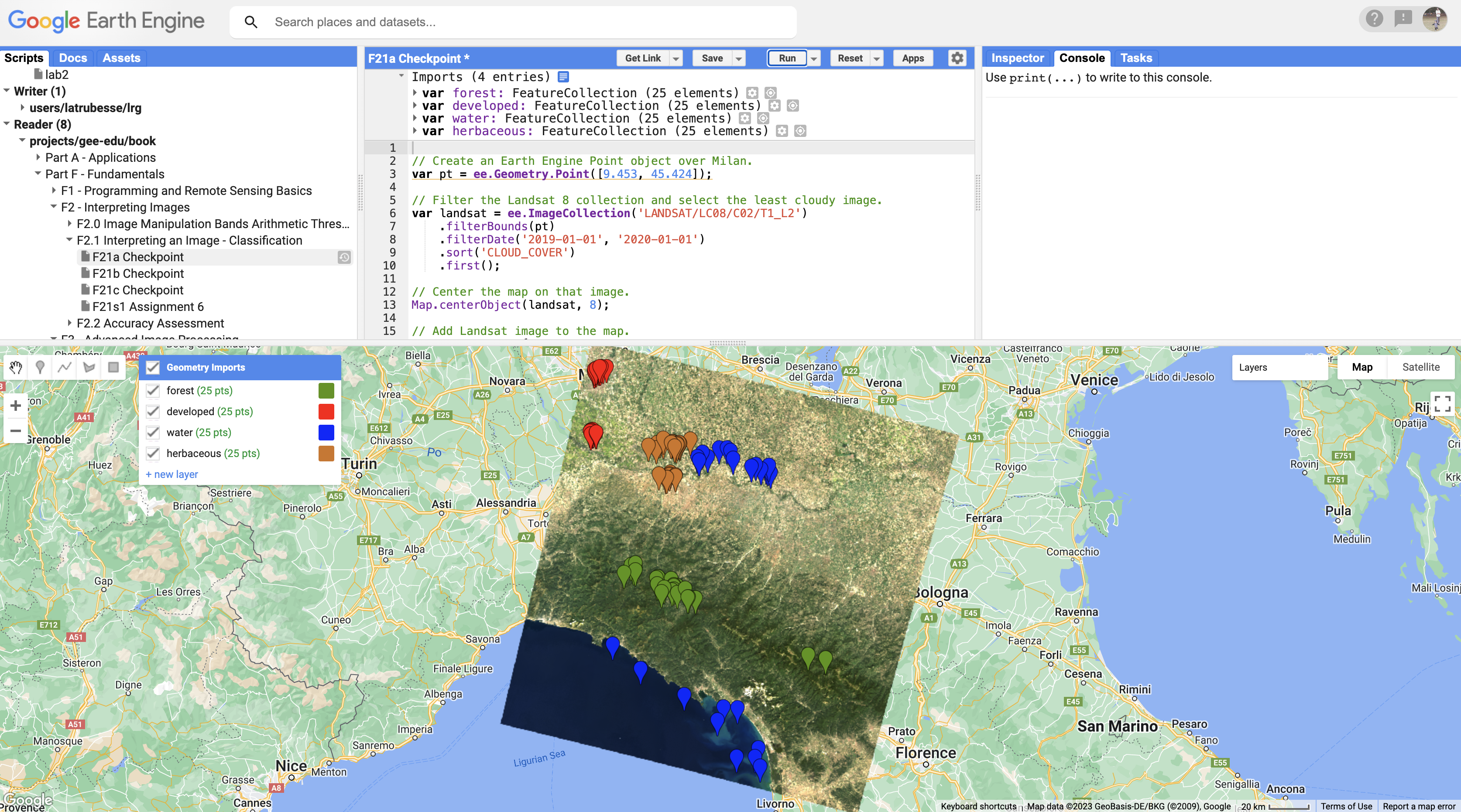
All four FeatureCollections with training points Try It
Use the satellite basemap to help identify land cover types, but base your point placement on how areas appear in the Landsat image itself. The classifier will learn from Landsat spectral values, not the basemap!
-
Part 4 - Combine Training Data
Merge all four FeatureCollections into one combined training dataset:
// Combine training feature collections.
var trainingFeatures = ee.FeatureCollection([
    forest, developed, water, herbaceous
]).flatten();

print('Training features:', trainingFeatures);
Understanding the code:
ee.FeatureCollection([...])- Creates a collection of collections.flatten()- Converts nested collections into one flat FeatureCollection
Verify in the Console that each feature has a
classproperty with values 0-3. -
Part 5 - Extract Spectral Information
Sample the Landsat band values at each training point location:
// Define prediction bands.
var predictionBands = [
    'SR_B1', 'SR_B2', 'SR_B3', 'SR_B4', 'SR_B5', 'SR_B6', 'SR_B7',
    'ST_B10'
];

// Sample training points.
var classifierTraining = Landsat.select(predictionBands)
    .sampleRegions({
        collection: trainingFeatures,
        properties: ['class'],
        scale: 30
    });

print('Sampled training data:', classifierTraining);
Understanding the code:
predictionBands- The spectral bands the classifier will use to learn patterns.sampleRegions()- Extracts pixel values at each point locationproperties: ['class']- Keeps the class label with each samplescale: 30- Matches Landsat's 30-meter resolution
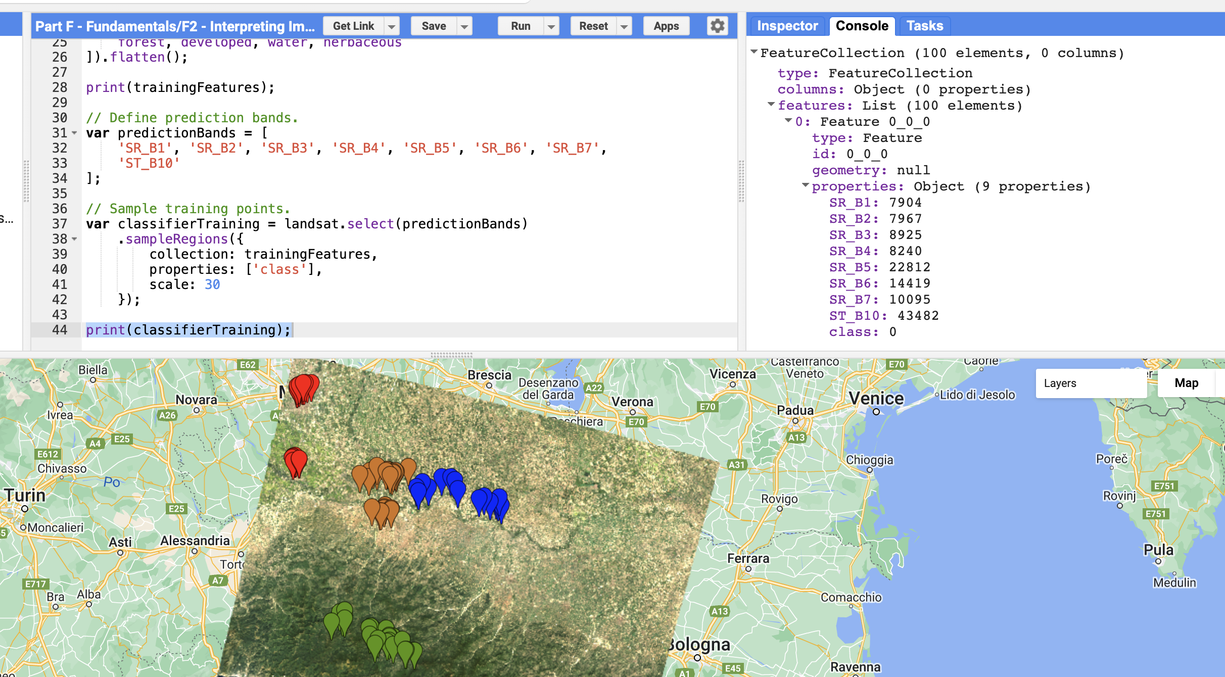
Each feature now has band values AND the class property -
Part 6 - Train a CART Classifier
CART (Classification and Regression Tree) is a decision tree algorithm that creates rules based on band values:
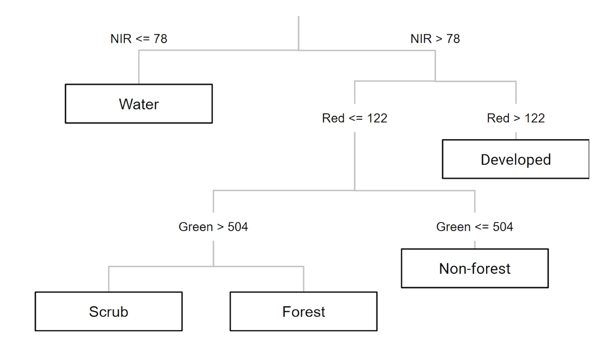
A decision tree creates if/then rules to classify pixels //////////////// CART Classifier /////////////////// // Train a CART Classifier. var classifier = ee.Classifier.smileCart().train({ features: classifierTraining, classProperty: 'class', inputProperties: predictionBands }); // View the decision rules print('CART decision tree:', classifier.explain());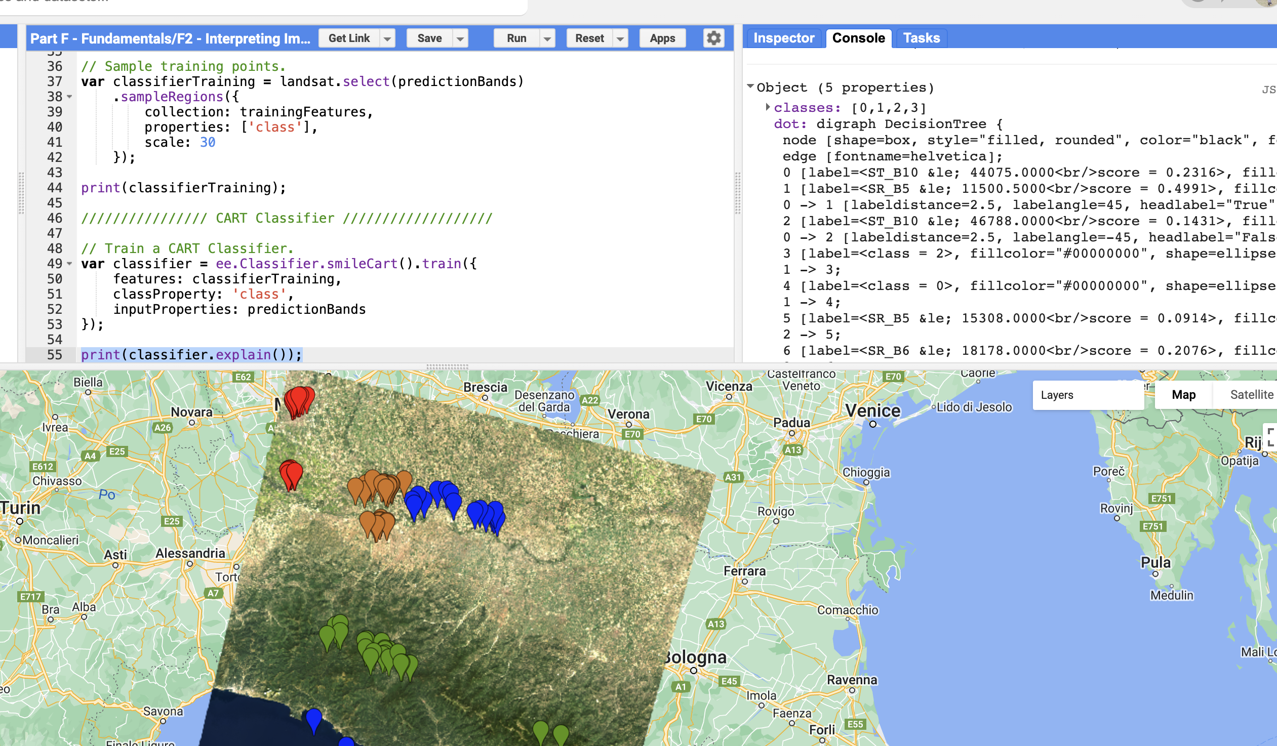
The "tree" property shows the decision rules -
Part 7 - Classify the Image
Apply the trained classifier to classify every pixel in the Landsat image:
// Classify the Landsat image.
var classified = Landsat.select(predictionBands).classify(classifier);

// Define classification image visualization parameters.
var classificationVis = {
    min: 0,
    max: 3,
    palette: ['589400', 'ff0000', '1a11ff', 'd0741e']
};

// Add the classified image to the map.
Map.addLayer(classified, classificationVis, 'CART classified');
Understanding the palette: The colors correspond to class values 0–3 in order: Forest (green), Developed (red), Water (blue), Herbaceous (orange).
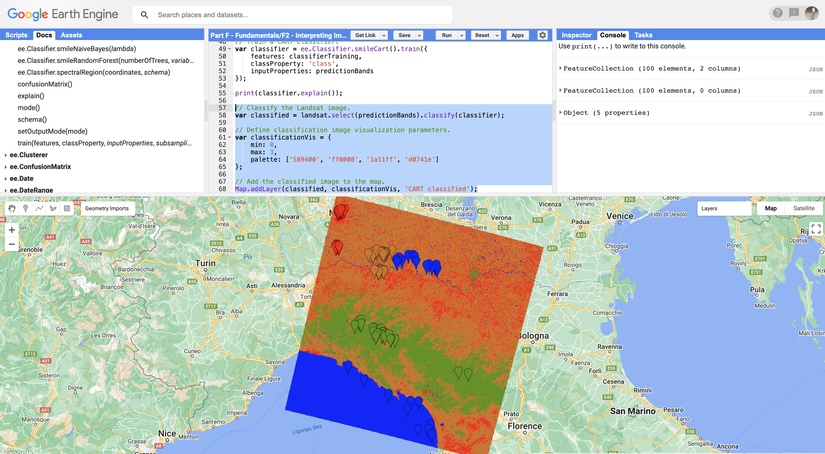
CART classification result for Milan area Try It
Toggle between the classified image and the original Landsat layer. Use the layer transparency slider to compare. Look for areas where the classification seems wrong.
-
Part 8 - Train a Random Forest Classifier
Random Forest builds many decision trees and uses voting to improve accuracy:
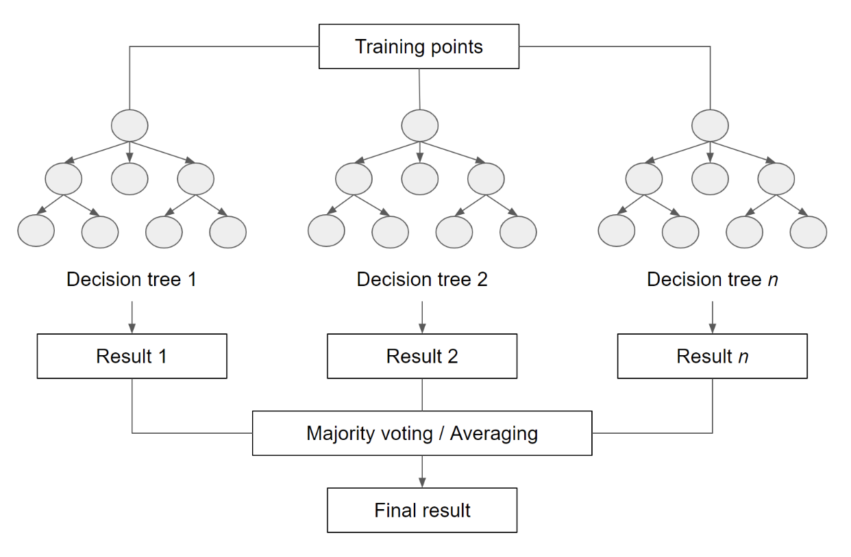
Random Forest combines many trees through voting /////////////// Random Forest Classifier ///////////////////// // Train RF classifier. var RFclassifier = ee.Classifier.smileRandomForest(50).train({ features: classifierTraining, classProperty: 'class', inputProperties: predictionBands }); // Classify Landsat image. var RFclassified = Landsat.select(predictionBands).classify(RFclassifier); // Add classified image to the map. Map.addLayer(RFclassified, classificationVis, 'RF classified');Understanding the code:
smileRandomForest(50)- Creates a Random Forest with 50 decision trees- More trees generally = better accuracy, but longer computation
- The
seedparameter (optional) makes results reproducible
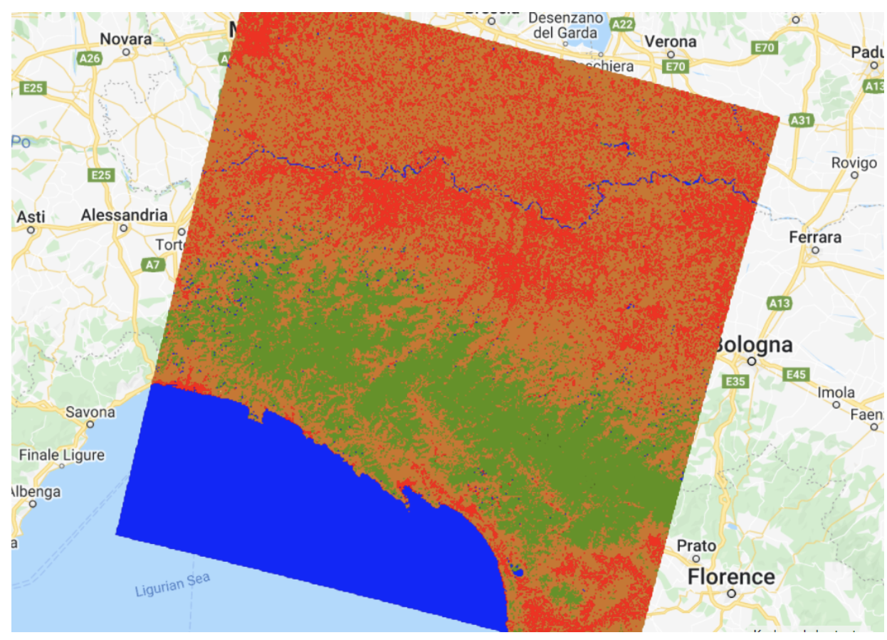
Random Forest classification result -
Part 9 - Compare and Analyze Results
Inspect both classifications and consider these questions:
- Which classifier produces smoother results?
- Where do you see obvious misclassifications?
- Which classes are most often confused with each other?
Ways to Improve Classification:
- Collect more training data: More points = better learning
- Tune hyperparameters: Adjust the number of trees or tree depth
- Try other classifiers: SVM, Gradient Tree Boost, etc.
- Distribute samples spatially: Cover the entire study area
- Add spectral indices: NDVI, NDWI can help separate vegetation from urban
Lab Instructions
Check Your Understanding
- Why do we use
.flatten()when combining FeatureCollections? - What does the
scale: 30parameter in sampleRegions represent? - Why might Random Forest perform better than a single decision tree?
- If your "Developed" class is being confused with "Herbaceous," what could you do?
Troubleshooting
Solution: Make sure you added a property named exactly class
(lowercase) when configuring each FeatureCollection. Check the gear icon settings.
Solution: You may need more training points. Aim for at least 25 per class, distributed across your entire study area.
Solution: Check that your class values (0, 1, 2, 3) are correct in each FeatureCollection. Also verify that classifierTraining actually contains samples from all classes.
Key Takeaways
- Supervised classification requires labeled training data YOU provide
- Use FeatureCollections with a
classproperty for training points sampleRegions()extracts band values at training point locations- CART creates a single decision tree (simple, interpretable)
- Random Forest uses many trees and voting (usually more accurate)
- Classification accuracy depends heavily on training data quality
Common Mistakes to Avoid
- Too few training points: Aim for 20–30+ samples per class
- Mixed pixels: Place points in homogeneous areas, not on edges between classes
- Wrong scale: Use
scale: 30for Landsat,scale: 10for Sentinel-2 - Forgetting the class property: Every FeatureCollection must have a
classfield - Points only in one area: Distribute training data across the entire image
Pro Tips
- Add spectral indices (NDVI, NDWI) as additional bands to improve classification
- Use high-resolution imagery in the basemap to verify your training points
- Random Forest with 50–100 trees usually provides good results
- Save your training points as an Asset so you don't lose them!
- Use
.randomColumn()to split data for training and validation
📋 Lab Submission
Subject: Lab 11 - Supervised Classification - [Your Name]
Include in your submission:
- Shareable link to your GEE script
- Question 1: How does the Random Forest classification differ from the CART classification?
- Question 2: Why do you think CART had more classification errors? How would you improve it?
- Question 3: Based on visual examination, which classifier performed better? Explain.
Add your answers as comments at the end of your code.