Part 1: Creating and Analyzing a Single River Mask

In this section, we will prepare an image and calculate some simple morphological attributes of a river. To do this, we will use a pre-classified image of surface water occurrence, identify which pixels represent the river and channel bars, and finally calculate the centerline, width, and bank characteristics.

You will need to start with a boilerplate script below. Copy and paste the code below into Google Earth Engine.

var aoi =
    /* color: #d63000 */
    /* shown: false */
    /* displayProperties: [
      {
        "type": "rectangle"
      }
    ] */
    ee.Geometry.Polygon(
      [[[-67.18414102495456, -11.09095257894929],
        [-67.18414102495456, -11.402427204567534],
        [-66.57886300981784, -11.402427204567534],
        [-66.57886300981784, -11.09095257894929]]], null, false);

var sword = ee.FeatureCollection("projects/gee-book/assets/A2-4/SWORD");

var getUTMProj = function(lon, lat) {
    // given longitude and latitude (in degree decimals) return EPSG string for the
    // corresponding UTM projection
    var utmCode = ee.Number(lon).add(180).divide(6).ceil().int();
    var output = ee.Algorithms.If(ee.Number(lat).gte(0),
        ee.String('EPSG:326').cat(utmCode.format('%02d')),
        ee.String('EPSG:327').cat(utmCode.format('%02d')));
    return (output);
};

var coords = aoi.centroid(30).coordinates();
var lon = coords.get(0);
var lat = coords.get(1);
var crs = getUTMProj(lon, lat);
var scale = ee.Number(30);

var rpj = function(image) {
    return image.reproject({
        crs: crs,
        scale: scale
    });
};

The script includes our example area of interest (aoi) and two helper functions for reprojecting data to the local UTM coordinates. We force this projection and scale for many of our map layers because we are trying to observe and measure the river morphology. As data is viewed at different zoom levels, the shapes and apparent connectivity of many water bodies will change. To allow a given dataset to be viewed with the same detail at multiple scales, we can force the data to be reprojected, as we do here.

The Joint Research Centre’s surface water occurrence dataset (Pekel et al. 2016) classified the entire Landsat 5, 7, and 8 histories and produced annual maps identifying seasonal and permanent water classes. Here, we will include both seasonal and permanent water classes (represented by pixel values of ≥2) as water pixels (with value = 1) and the rest as non-water pixels (with value = 0). In this section, we will look at only one image at a time by choosing the image from the year 2000. Copy and paste the code below, bg is a dark background layer for other map layers to be easily seen.

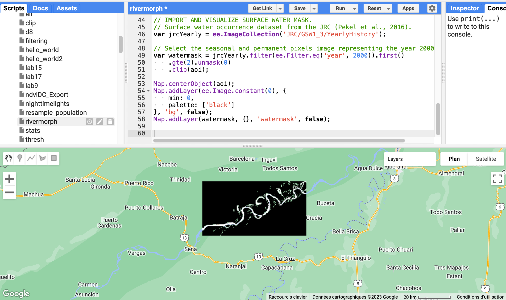
// IMPORT AND VISUALIZE SURFACE WATER MASK.
// Surface water occurrence dataset from the JRC (Pekel et al., 2016).
var jrcYearly = ee.ImageCollection('JRC/GSW1_3/YearlyHistory');

// Select the seasonal and permanent pixels image representing the year 2000
var waterMask = jrcYearly.filter(ee.Filter.eq('year', 2000)).first()
    .gte(2).unmask(0)
    .clip(aoi);

Map.centerObject(aoi);
Map.addLayer(ee.Image.constant(0), {
    min: 0,
    palette: ['black']
}, 'bg', false);
Map.addLayer(waterMask, {}, 'water mask', false);

Next, we clean up the water mask by filling in small gaps by performing a closing operation (dilation followed by erosion). Areas of non-water pixels inside surface water bodies in the water mask may represent small channel bars, which we will fill to create a simplified water mask. We identify these bars using vectorization; however, you could do a similar operation with the connectedPixelCount method for bars up to 256 pixels in size. Filling in these small bars in the river mask improves the creation of a new centerline later in the lab.

// REMOVE NOISE AND SMALL ISLANDS TO SIMPLIFY THE TOPOLOGY.
// a. Image closure operation to fill small holes.
waterMask = waterMask.focal_max().focal_min();

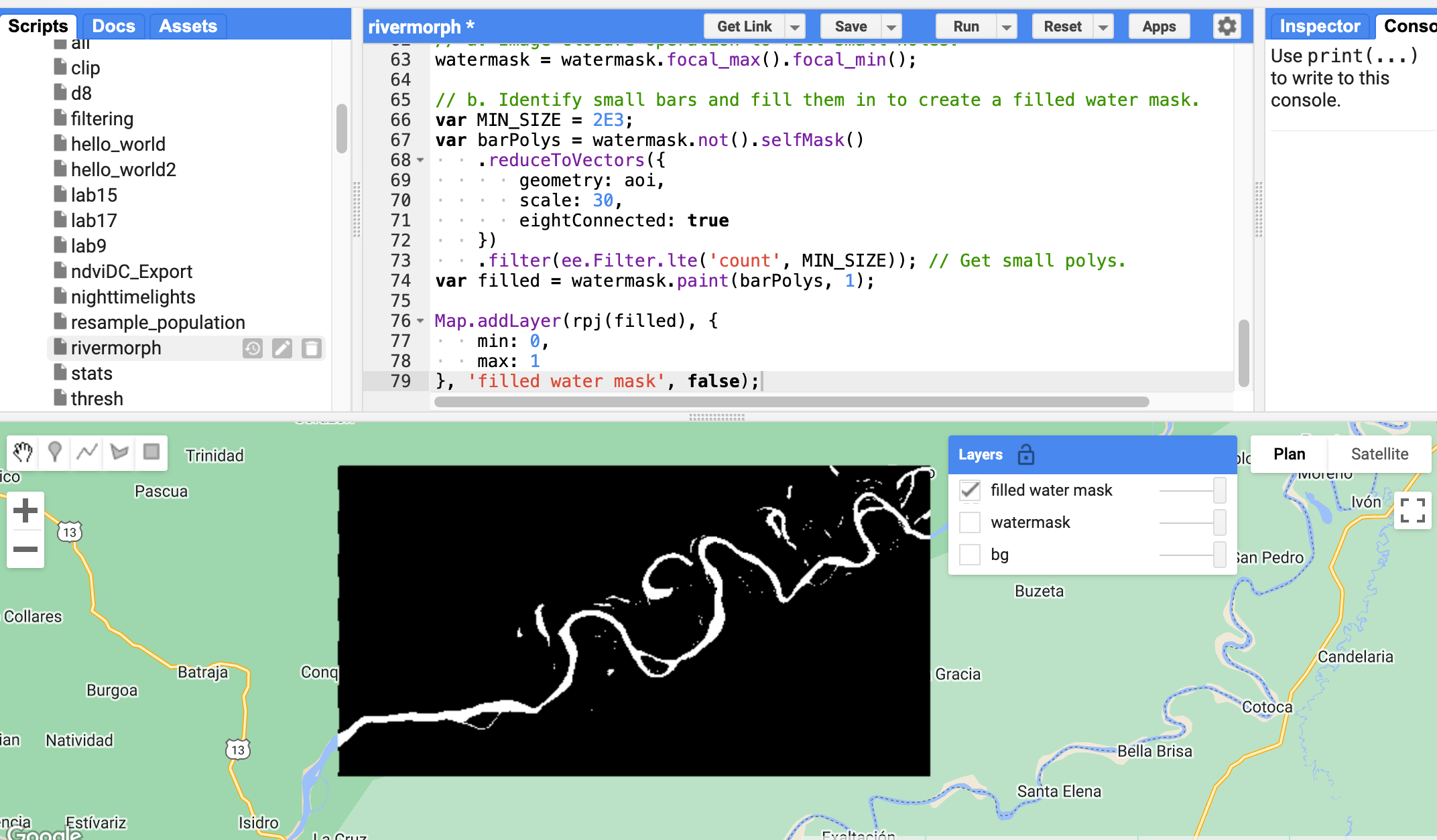
// b. Identify small bars and fill them in to create a filled water mask.
var MIN_SIZE = 2E3;
var barPolys = waterMask.not().selfMask()
    .reduceToVectors({
        geometry: aoi,
        scale: 30,
        eightConnected: true
    })
    .filter(ee.Filter.lte('count', MIN_SIZE)); // Get small polys.
var filled = waterMask.paint(barPolys, 1);

Map.addLayer(rpj(filled), {
    min: 0,
    max: 1
}, 'filled water mask', false);

We forced reprojection of the map layer using the helper function rpj. This means we must be careful to keep our domain small enough to be processed at the set scale when calculating on the fly in the Code Editor; otherwise, we will run out of memory. The reprojection may not be necessary when exporting the output using a task.

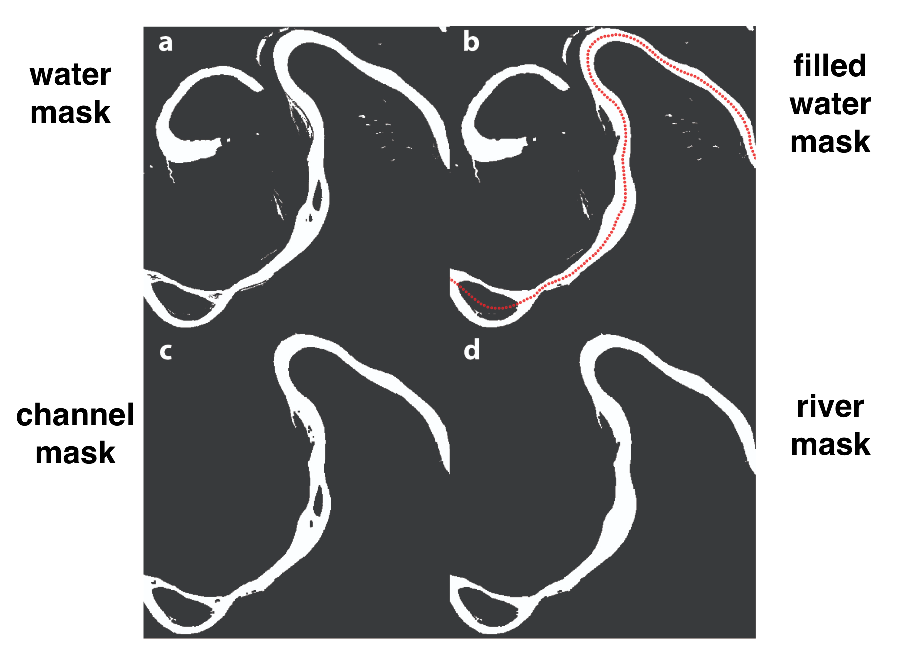
In the following step, we extract water bodies in the water mask corresponding to rivers. We will define a river mask (Figure D) to be pixels connected to the river centerline according to the filled water mask. The channel mask (Figure C) is also defined by connectivity but excludes the small bars, giving us more accurate widths and areas for change detection in later sections.

We can extract the river mask by checking the water pixels’ connectivity to a provided river location database. Specifically, we use the Earth Engine method cumulativeCost to identify connectivity between the filled water mask and the pixels corresponding to the river dataset. By inverting the filled mask, the cost to traverse water pixels is 0, and the cost over land pixels is 1. Pixels in the cost map with a value of 0 are entirely connected to the Surface Water and Ocean Topography (SWOT) Mission River Database (SWORD) centerline points by water, and pixels with values greater than 0 are separated from SWORD by land. The SWORD data, which were loaded as assets in the starter script, have some points located on land, either because the channel bifurcates or because the channel has migrated, so we must exclude those from our cumulative cost parameter source, or they will appear as single pixels of 0 in our cost map.

The maxDistance parameter must be set to capture the maximum distance between centerline points and river pixels. In a single-threaded river with an accurate centerline, the ideal maxDistance value would be about half the river width. However, in reality, the centerlines are not perfect, and large islands may separate pixels from their nearest centerline. Unfortunately, increasing maxDistance has a large computational penalty, so some tweaking is required to get an optimal value. We can set geodeticDistance to false to regain some computational efficiency, because we are not worried about the accuracy of the distances.

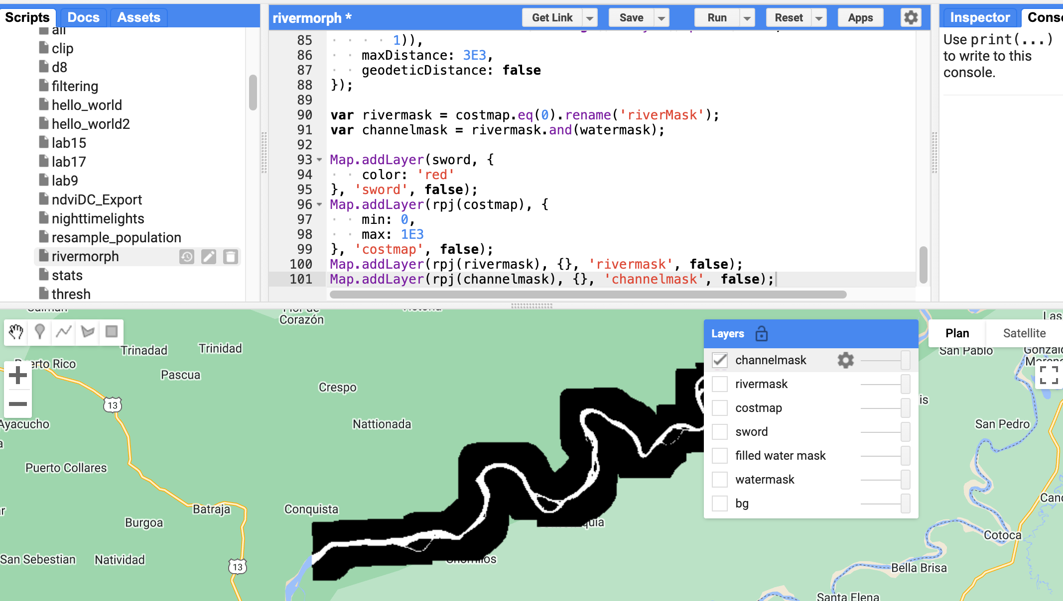
// IDENTIFYING RIVERS FROM OTHER TYPES OF WATER BODIES.
// Cumulative cost mapping to find pixels connected to a reference centerline.
var costmap = filled.not().cumulativeCost({
    source: waterMask.and(ee.Image().toByte().paint(sword,
        1)),
    maxDistance: 3E3,
    geodeticDistance: false
});

var rivermask = costmap.eq(0).rename('riverMask');
var channelmask = rivermask.and(waterMask);

Map.addLayer(sword, {
    color: 'red'
}, 'sword', false);
Map.addLayer(rpj(costmap), {
    min: 0,
    max: 1E3
}, 'costmap', false);
Map.addLayer(rpj(rivermask), {}, 'rivermask', false);
Map.addLayer(rpj(channelmask), {}, 'channelmask', false);

Your code up to this point should look like this:

var aoi =
    /* color: #d63000 */
    /* shown: false */
    /* displayProperties: [
      {
        "type": "rectangle"
      }
    ] */
    ee.Geometry.Polygon(
      [[[-67.18414102495456, -11.09095257894929],
        [-67.18414102495456, -11.402427204567534],
        [-66.57886300981784, -11.402427204567534],
        [-66.57886300981784, -11.09095257894929]]], null, false);

var sword = ee.FeatureCollection("projects/gee-book/assets/A2-4/SWORD");

var getUTMProj = function(lon, lat) {
    var utmCode = ee.Number(lon).add(180).divide(6).ceil().int();
    var output = ee.Algorithms.If(ee.Number(lat).gte(0),
        ee.String('EPSG:326').cat(utmCode.format('%02d')),
        ee.String('EPSG:327').cat(utmCode.format('%02d')));
    return (output);
};

var coords = aoi.centroid(30).coordinates();
var lon = coords.get(0);
var lat = coords.get(1);
var crs = getUTMProj(lon, lat);
var scale = ee.Number(30);

var rpj = function(image) {
    return image.reproject({
        crs: crs,
        scale: scale
    });
};

// IMPORT AND VISUALIZE SURFACE WATER MASK.
var jrcYearly = ee.ImageCollection('JRC/GSW1_3/YearlyHistory');
var waterMask = jrcYearly.filter(ee.Filter.eq('year', 2000)).first()
    .gte(2).unmask(0)
    .clip(aoi);
Map.centerObject(aoi);
Map.addLayer(ee.Image.constant(0), {
    min: 0,
    palette: ['black']
}, 'bg', false);
Map.addLayer(waterMask, {}, 'water mask', false);

// REMOVE NOISE AND SMALL ISLANDS TO SIMPLIFY THE TOPOLOGY.
waterMask = waterMask.focal_max().focal_min();
var MIN_SIZE = 2E3;
var barPolys = waterMask.not().selfMask()
    .reduceToVectors({
        geometry: aoi,
        scale: 30,
        eightConnected: true
    })
    .filter(ee.Filter.lte('count', MIN_SIZE));
var filled = waterMask.paint(barPolys, 1);
Map.addLayer(rpj(filled), {
    min: 0,
    max: 1
}, 'filled water mask', false);

// IDENTIFYING RIVERS FROM OTHER TYPES OF WATER BODIES.
var costmap = filled.not().cumulativeCost({
    source: waterMask.and(ee.Image().toByte().paint(sword,
        1)),
    maxDistance: 3E3,
    geodeticDistance: false
});
var rivermask = costmap.eq(0).rename('riverMask');
var channelmask = rivermask.and(waterMask);
Map.addLayer(sword, {
    color: 'red'
}, 'sword', false);
Map.addLayer(rpj(costmap), {
    min: 0,
    max: 1E3
}, 'costmap', false);
Map.addLayer(rpj(rivermask), {}, 'rivermask', false);
Map.addLayer(rpj(channelmask), {}, 'channelmask', false);