Part 5: Riverback Erosion

In this part, we return to the Madre de Dios River as our study area. We will apply the methods we developed in Parts 1-3 to multiple images, calculate the amount of bank erosion, and summarize our results onto our centerline. Before doing so, we will create a new script that wraps the masking and morphology code in Parts 1-3 into a function called makeChannelmask with one argument for the year. We return an image with bands for all the masks and bank calculations, plus a property named 'year' containing the year argument.

//redefining the variables to prevent errors
var jrcYearly = ee.ImageCollection("JRC/GSW1_3/YearlyHistory"),
    aoi = ee.Geometry.Polygon(
      [[[-66.75498758257174, -11.090110301403685],
        [-66.75498758257174, -11.258517279582335],
        [-66.56650339067721, -11.258517279582335],
        [-66.56650339067721, -11.090110301403685]]], null, false),
    sword = ee.FeatureCollection("projects/gee-book/assets/A2-4/SWORD");

var getUTMProj = function(lon, lat) {
    var utmCode = ee.Number(lon).add(180).divide(6).ceil().int();
    var output = ee.Algorithms.If({
        condition: ee.Number(lat).gte(0),
        trueCase: ee.String('EPSG:326').cat(utmCode.format('%02d')),
        falseCase: ee.String('EPSG:327').cat(utmCode.format('%02d'))
    });
    return (output);
};

var coords = aoi.centroid(30).coordinates();
var lon = coords.get(0);
var lat = coords.get(1);
var crs = getUTMProj(lon, lat);
var scale = 30;

var rpj = function(image) {
    return image.reproject({
        crs: crs,
        scale: scale
    });
};

var distanceKernel = ee.Kernel.euclidean({
    radius: 30,
    units: 'meters',
    magnitude: 0.5
});

var makeChannelmask = function(year) {
    var waterMask = jrcYearly.filter(ee.Filter.eq('year', year))
        .first()
        .gte(2).unmask()
        .focal_max().focal_min()
        .rename('waterMask');

    var barPolys = waterMask.not().selfMask()
        .reduceToVectors({
            geometry: aoi,
            scale: 30,
            eightConnected: false
        })
        .filter(ee.Filter.lte('count', 1E4)); // Get small polys.

    var filled = waterMask.paint(barPolys, 1).rename('filled');

    var costmap = filled.not().cumulativeCost({
        source: waterMask.and(ee.Image().toByte().paint(
            sword, 1)),
        maxDistance: 5E3,
        geodeticDistance: false
    }).rename('costmap');

    var rivermask = costmap.eq(0).rename('rivermask');
    var channelmask = rivermask.and(waterMask).rename('channelmask');

    var bankMask = channelmask.focal_max(1).neq(channelmask)
        .rename('bankMask');
    var bankDistance = channelmask.not().cumulativeCost({
        source: channelmask,
        maxDistance: 1E2,
        geodeticDistance: false
    });
    var bankAspect = ee.Terrain.aspect(bankDistance).mask(
        bankMask).rename('bankAspect');

    var bankLength = bankMask.convolve(distanceKernel)
        .mask(bankMask).rename('bankLength');

    return ee.Image.cat([
        waterMask, channelmask, rivermask, bankMask,
        bankAspect, bankLength
    ]).set('year', year)
      .clip(aoi);
};

Change Detection

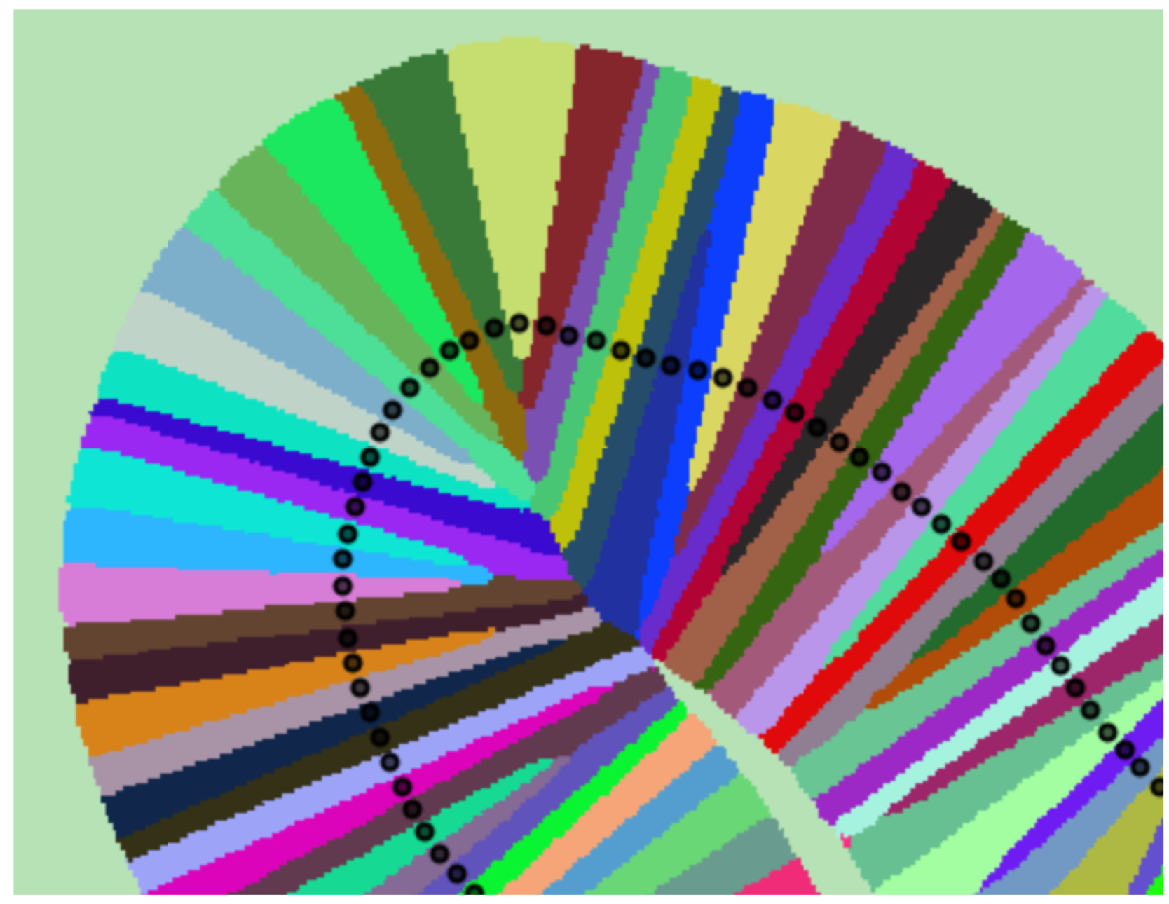
For this example, we use a section of the Madre de Dios River as our study area because it migrates more quickly, more than 30 m per year in some locations. Our methods work best if the two channel masks partially overlap everywhere along the length of the river; if there is a gap between the two masks, we will underestimate the amount of change and cannot calculate the change direction. We pick the years 2015 and 2020 for our example. We first create these two sets of channel masks and add them to the map (Fig. A2.4.4a).

var masks1 = makeChannelmask(2015);
var masks2 = makeChannelmask(2020);
Map.centerObject(aoi, 13);
var year1mask = rpj(masks1.select('channelmask').selfMask());
Map.addLayer(year1mask, {
    palette: ['blue']
}, 'year 1');
var year2mask = rpj(masks2.select('channelmask').selfMask());
Map.addLayer(year2mask, {
    palette: ['red']
}, 'year 2', true, 0.5);

Fig. A single meander bend of the Madre de Dios River in Bolivia, showing areas of erosion and accretion: (a) channel mask from 2015 in blue and channel mask from 2020 in red at 50% transparency; (b) pixels that represent erosion between 2015 and 2020

Erosion Calculation

Next, we create an image to represent the eroded area (Fig. A2.4.4b). We can quickly calculate this by comparing the channel mask in year 2 to the inverse water mask from year 1.

// Pixels that are now the river channel but were previously land.
erosion = masks2.select('channelmask')
    .and(masks1.select('waterMask').not())
    .rename('erosion');
Map.addLayer(rpj(erosion).selfMask(), {}, 'erosion', false);

Erosion Direction

Now we approximate the direction of erosion by the shortest path through the eroded area from each bank pixel in year 1 to any of the bank pixels in year 2. We use Image.cumulativeCost to measure the distance using the erosion image as our cost surface.

// Erosion distance assuming the shortest distance between banks.
erosionEndpoints = erosion.focal_max(1).and(masks2.select('bankMask'));
erosionDistance = erosion.focal_max(1).selfMask()
    .cumulativeCost({
        source: erosionEndpoints,
        maxDistance: 1E3,
        geodeticDistance: true
    }).rename('erosionDistance');
Map.addLayer(rpj(erosionDistance), {
    min: 0,
    max: 300
}, 'erosion distance', false);

// Direction of the erosion following slope of distance.
erosionDirection = ee.Terrain.aspect(erosionDistance)
    .multiply(Math.PI).divide(180)
    .clip(aoi)
    .rename('erosionDirection');
erosionDistance = erosionDistance.mask(erosion);
Map.addLayer(rpj(erosionDirection), {
    min: 0,
    max: Math.PI
}, 'erosion direction', false);

Connecting to the Centerline

We now have all our change metrics calculated as images in Earth Engine. To analyze a lot of river data, we often want to look at long profiles of river or tributary networks in a watershed. To do this, we use reducers to summarize our raster data back onto our vector centerline.

// Distance to nearest SWORD centerline point.
distance = sword.distance(2E3).clip(aoi);
// Second derivatives of distance.
concavityBounds = distance.convolve(ee.Kernel.laplacian8())
    .gte(0).rename('bounds');
Map.addLayer(rpj(distance), {
    min: 0,
    max: 1E3
}, 'distance', false);
Map.addLayer(rpj(concavityBounds), {}, 'bounds', false);

Node Assignment and Data Summarization

// Reduce the pixels according to the concavity boundaries, and set the value to SWORD node ID.
swordImg = ee.Image(0).paint(sword, 'node_id').rename('node_id')
    .clip(aoi);
nodePixels = concavityBounds.addBands(swordImg)
    .reduceConnectedComponents({
        reducer: ee.Reducer.max(),
        labelBand: 'bounds'
    }).focalMode({
        radius: 3,
        iterations: 2
    });
Map.addLayer(rpj(nodePixels).randomVisualizer(), {}, 'node assignments', false);

Summarizing the Data

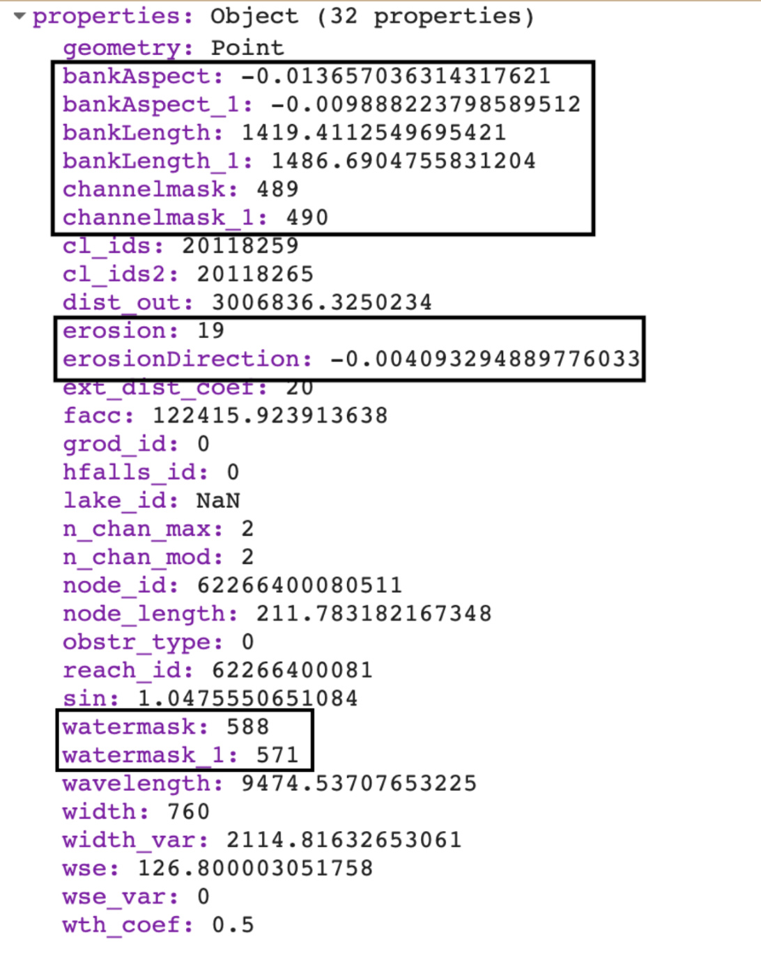
The final step is to apply a reducer that uses our nodePixels image from the previous step to group our raster data. We combine the reducer.forEach and reducer.group methods into our own custom function that we can use with different reducers to get our final results. The grouped reducers in our function return a list of dictionaries. We map over the list and create a FeatureCollection before returning from the function.

// Set up a custom reducing function to summarize the data.
var groupReduce = function(dataImg, nodeIds, reducer) {
    var groupReducer = reducer.forEach(dataImg.bandNames())
        .group({
            groupField: dataImg.bandNames().length(),
            groupName: 'node_id'
        });
    var statsList = dataImg.addBands(nodeIds).clip(aoi)
        .reduceRegion({
            reducer: groupReducer,
            scale: 30,
        }).get('groups');
    var statsOut = ee.List(statsList).map(function(dict) {
        return ee.Feature(null, dict);
    });
    return ee.FeatureCollection(statsOut);
};

dataMask = masks1.addBands(masks2).reduce(ee.Reducer.anyNonZero());
sumBands = ['waterMask', 'channelmask', 'bankLength'];
sumImg = erosion.addBands(masks1, sumBands)
    .addBands(masks2, sumBands);
sumStats = groupReduce(sumImg, nodePixels, ee.Reducer.sum());

angleImg = erosionDirection.addBands(masks1, ['bankAspect'])
    .addBands(masks2, ['bankAspect']);
angleStats = groupReduce(angleImg, nodePixels, ee.Reducer.circularMean());

vectorData = sword.filterBounds(aoi).map(function(feat) {
    var nodeFilter = ee.Filter.eq('node_id', feat.get('node_id'));
    var sumFeat = sumStats.filter(nodeFilter).first();
    var angleFeat = angleStats.filter(nodeFilter).first();
    return feat.copyProperties(sumFeat).copyProperties(angleFeat);
});

print(vectorData);
Map.addLayer(vectorData, {}, 'final data');

Based on raster calculations, this workflow can add many new properties to the river centerlines. For example, we calculated the amount of erosion between these two years, but you could use a similar code to calculate the amount of accretion. Other interesting river properties, like the banks' slope from a DEM, could be calculated and added to our centerline dataset.

Continue and submit your final code.