Global Snow Observatory: Trend Analysis

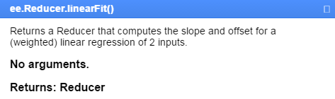
GEE has many built-in functions and operations for users to call, and luckily, a linear fit is among them. If you search for Linear in the documentation, we can see that ee.Reducer.linearFit() takes two inputs and returns a reducer.

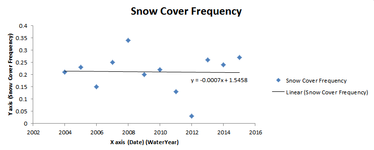
In this final step, we will perform that trend analysis. To do this, we must add a date time stamp to have the appropriate X value (time) for our Y value (Snow cover frequency).

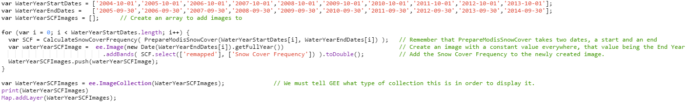
To add the date, we will also encompass all the other functions up to this point as well, because we need to format the newly created image collection correctly for the linearFit reducer. We will, therefore, create 3 arrays. One will contain the start dates, one the end dates and the other will be left blank. We will then iterate through the arrays in a for loop, using our previously created functions to calculate snow cover frequency. We will then use the data to create a band of constant value and add to that the snow cover frequency. The code to do this appears as follows:

// ...existing code for joining, masking, reclassifying, and calculating snow cover frequency...
var WaterYearStartDates = ['2004-10-01','2005-10-01','2006-10-01','2007-10-01','2008-10-01','2009-10-01','2010-10-01','2011-10-01','2012-10-01','2013-10-01'];
var WaterYearEndDates = ['2005-09-30','2006-09-30','2007-09-30','2008-09-30','2009-09-30','2010-09-30','2011-09-30','2012-09-30','2013-09-30','2014-09-30'];
var WaterYearSCFImages = [];
for (var i = 0; i < WaterYearStartDates.length; i++) {
  var SCF = CalculateSnowCoverFrequency( PrepareModisSnowCover(WaterYearStartDates[i], WaterYearEndDates[i]) );
  var waterYearSCFImage = ee.Image(new Date(WaterYearEndDates[i]).getFullYear())
    .addBands( SCF.select(['remapped'], ['Snow Cover Frequency']) ).toDouble();
  WaterYearSCFImages.push(waterYearSCFImage);
}
var WaterYearSCFImages = ee.ImageCollection(WaterYearSCFImages);
print(WaterYearSCFImages);
Map.addLayer(WaterYearSCFImages);

Earth Engine Code Example

This can be complicated to follow, so understand what we just did. If necessary, you can hand it a single set of dates and examine a single image in the collection. Once you are satisfied you understand what we just did, we will then apply the linear fit reducer. This call looks like such:

Earth Engine Code Example

After we run our reducer, it returns an image with two bands, one called 'scale' and one called 'offset'. This is Google's terms for 'slope' and 'intercept'. We are interested in the slope, so I added the 'scale' (slope) band to the map. Go ahead and run the code from the image directly above. What does the map look like?

Our map looks a little black. If you use the inspector on an area, you can see why. The range of the slopes is extremely small.