Deriving Land Surface Temperature from Landsat

Working with MODIS LST is relatively simple because the NASA team already processes the data. You can also derive LST from Landsat, which has a much finer native resolution (between ~60 m and ~120 m depending on the satellite) than the ~1 km MODIS pixels. However, you need to derive LST yourself from the measurements in the thermal bands, which usually involves some surface emissivity estimate (Li et al. 2013). The surface emissivity (ε) of a material is the effectiveness with which it can emit thermal radiation compared to a black body at the same temperature and can range from 0 (for a perfect reflector) to 1 (for a perfect absorber and emitter). Since the thermal radiation captured by satellites is a function of both LST and ε, you need to accurately prescribe or estimate ε to get to the correct LST. Let’s consider one such simple method using Landsat 8 data.

We will start by loading in the Landsat data, cloud screening, and filtering to a time and region of interest. Continuing in the same script from part 1, add the following code:

// Function to filter out cloudy pixels.
function cloudMask(cloudyScene) {
  // Add a cloud score band to the image.
  var scored = ee.Algorithms.Landsat.simpleCloudScore(cloudyScene);
  // Create an image mask from the cloud score band and specify threshold.
  var mask = scored.select(['cloud']).lte(10);
  // Apply the mask to the original image and return the masked image.
  return cloudyScene.updateMask(mask);
}

// Load the collection, apply cloud mask, and filter to date and region of interest.
var col = ee.ImageCollection('LANDSAT/LC08/C02/T1_TOA')
  .filterBounds(regionInt)
  .filterDate('2014-01-01', '2019-01-01')
  .filter(sumFilter)
  .map(cloudMask);

print('Landsat collection', col);

After creating a median composite as a simple way to further reduce the influence of clouds, we mask out the water pixels and select the brightness temperature band.

// Generate median composite.
var image = col.median();

// Select thermal band 10 (with brightness temperature).
var thermal = image.select('B10')
  .clip(regionInt)
  .updateMask(notWater);

Map.addLayer(thermal, {
    min: 295,
    max: 310,
    palette: ['blue', 'white', 'red']
  },
  'Landsat_BT');

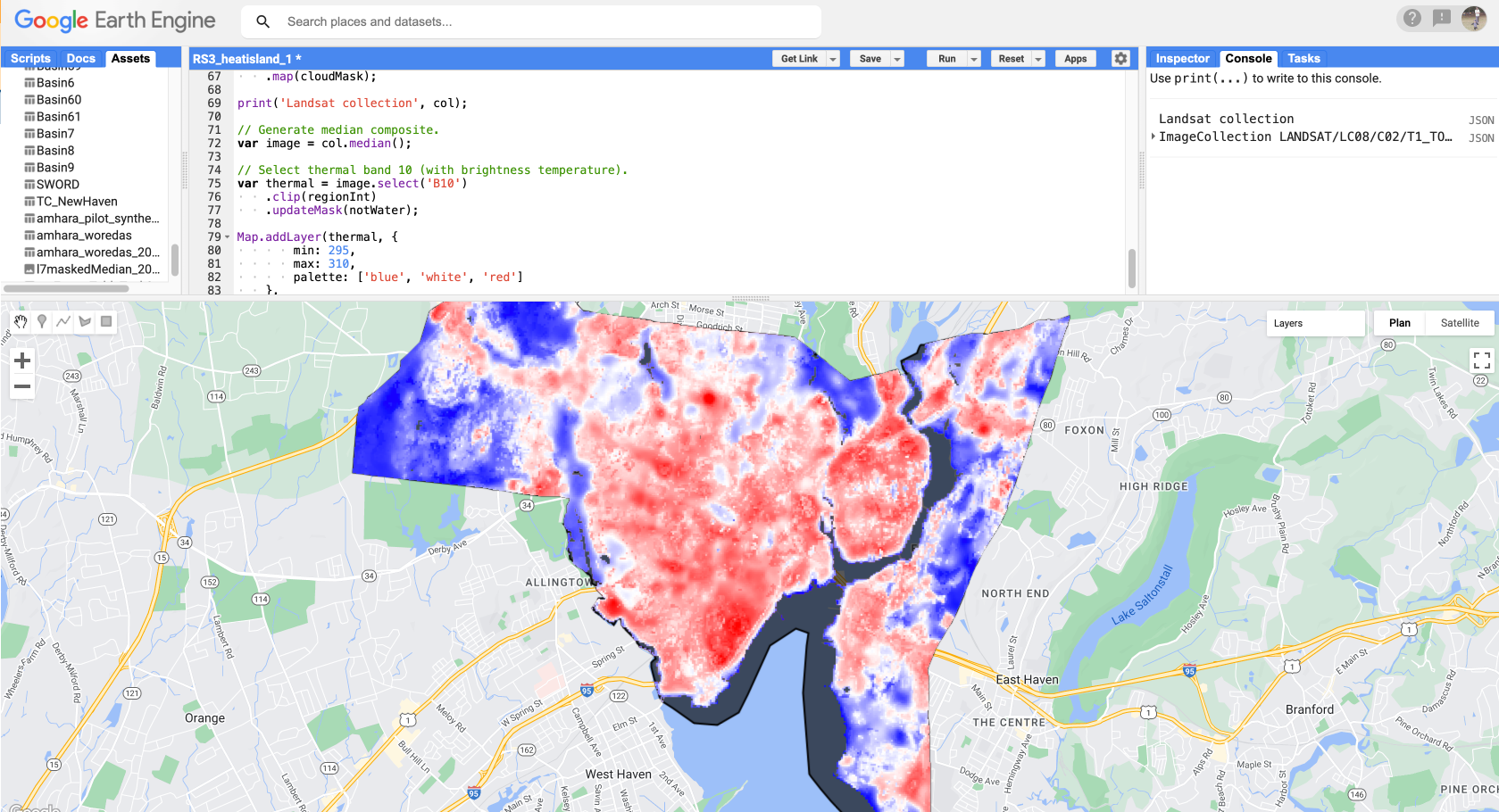
Brightness temperature is the equivalent of the infrared radiation escaping the top of the atmosphere, assuming the Earth to be a black body. It is not the same as the LST, which requires accounting for atmospheric absorption and re-emission, as well as the emissivity of the land surface. One way to derive pixel-level emissivity is as a function of the vegetation fraction of the pixel (Malakar et al. 2018). We start by calculating the Normalized Difference Vegetation Index (NDVI) from the Landsat surface reflectance data.

// Calculate NDVI from Landsat surface reflectance.
var ndvi = ee.ImageCollection('LANDSAT/LC08/C02/T1_L2')
  .filterBounds(regionInt)
  .filterDate('2014-01-01', '2019-01-01')
  .filter(sumFilter)
  .median()
  .normalizedDifference(['SR_B5', 'SR_B4']).rename('NDVI')
  .clip(regionInt)
  .updateMask(notWater);

Map.addLayer(ndvi, {
    min: 0,
    max: 1,
    palette: ['blue', 'white', 'green']
  },
  'ndvi');

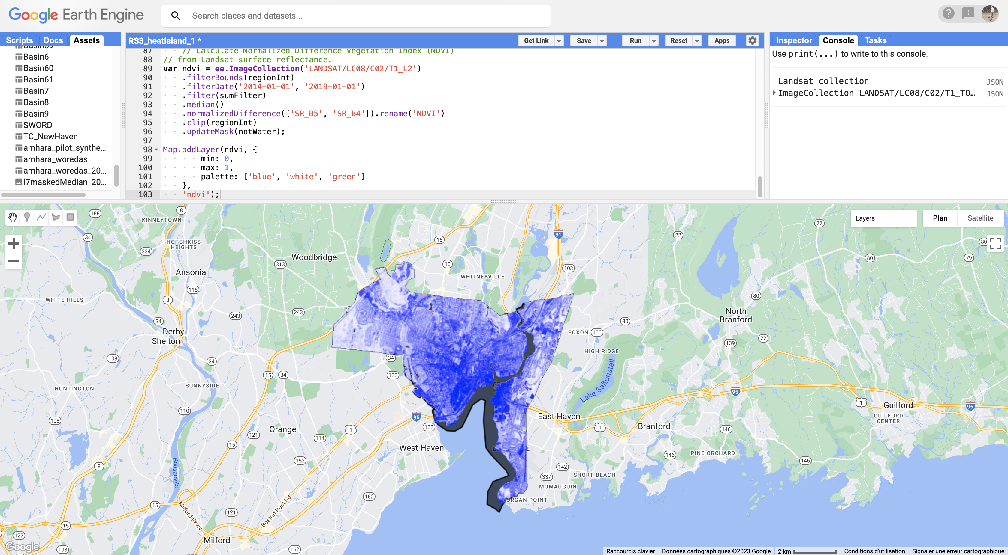
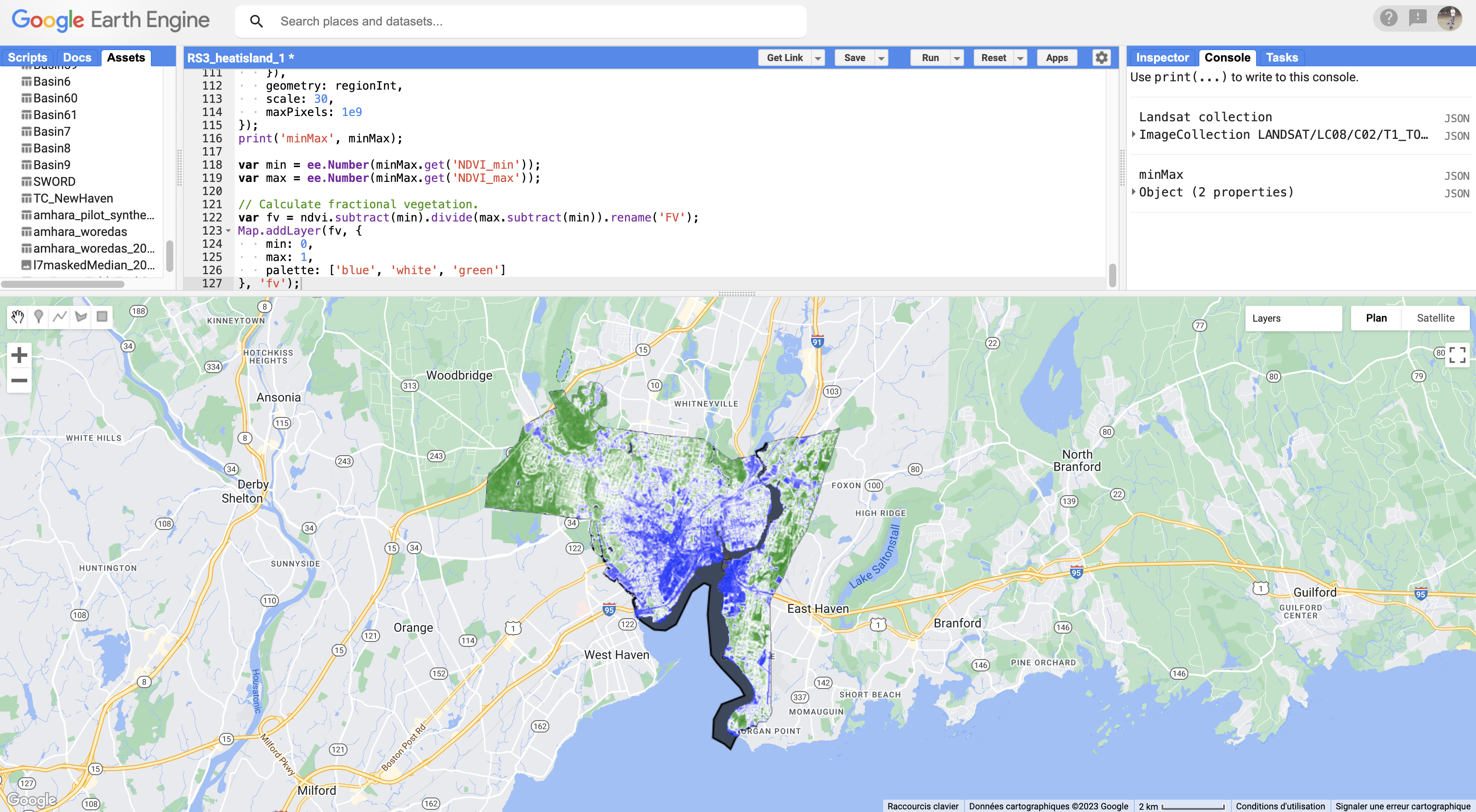
To map NDVI for each pixel to the actual fraction of the pixel with vegetation (fractional vegetation cover), we next use a relationship based on the range of NDVI values for each pixel.

// Find the minimum and maximum of NDVI.
var minMax = ndvi.reduceRegion({
  reducer: ee.Reducer.min().combine({
    reducer2: ee.Reducer.max(),
    sharedInputs: true
  }),
  geometry: regionInt,
  scale: 30,
  maxPixels: 1e9
});
var min = ee.Number(minMax.get('NDVI_min'));
var max = ee.Number(minMax.get('NDVI_max'));

// Calculate fractional vegetation.
var fv = ndvi.subtract(min).divide(max.subtract(min)).rename('FV');
Map.addLayer(fv, {
    min: 0,
    max: 1,
    palette: ['blue', 'white', 'green']
  },
  'fv');

Now, we use an empirical emissivity model based on this fractional vegetation cover (Sekertekin and Bonafoni 2020).

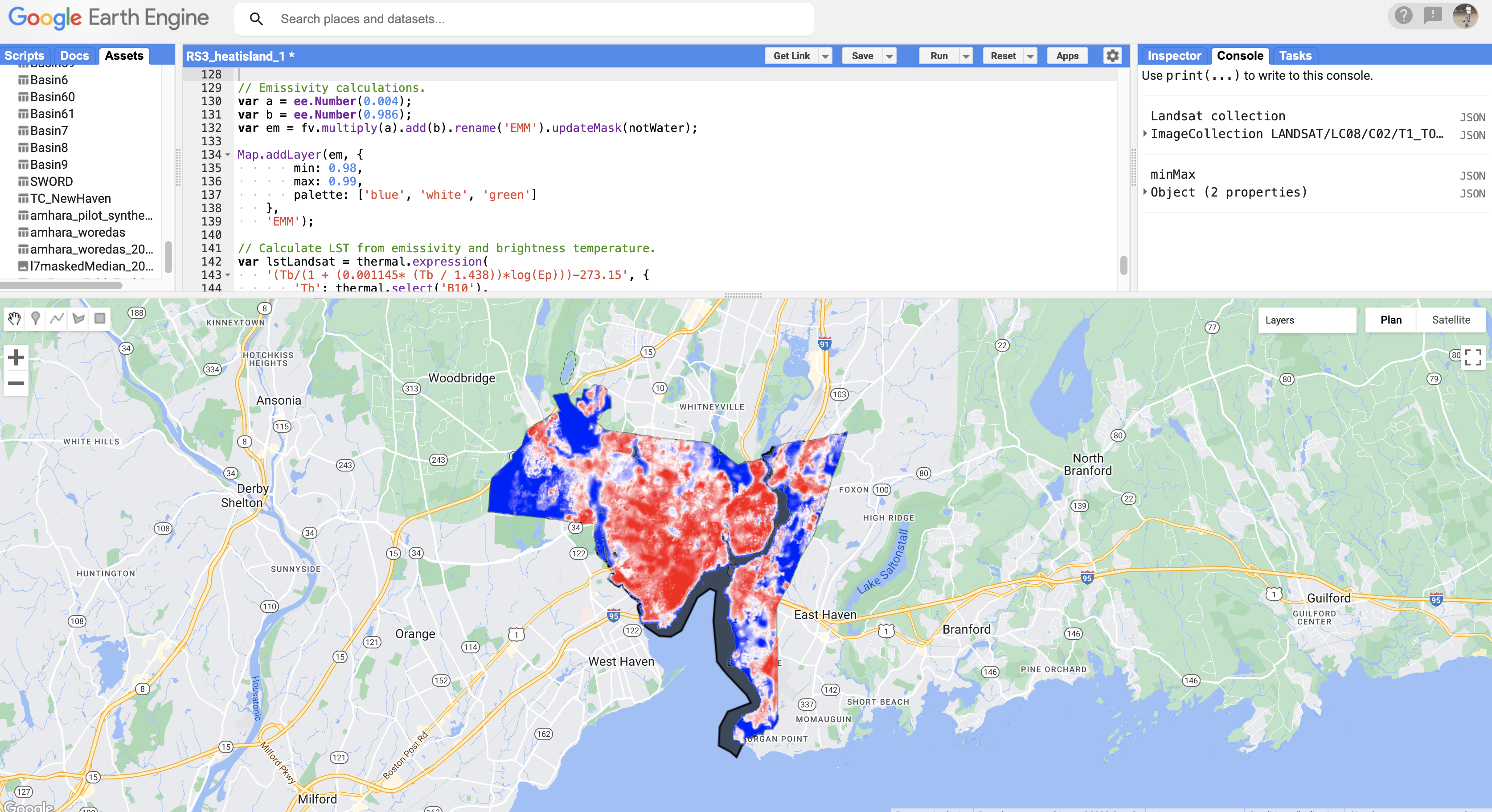
// Emissivity calculations.
var a = ee.Number(0.004);
var b = ee.Number(0.986);
var em = fv.multiply(a).add(b).rename('EMM').updateMask(notWater);
Map.addLayer(em, {
    min: 0.98,
    max: 0.99,
    palette: ['blue', 'white', 'green']
  },
  'EMM');

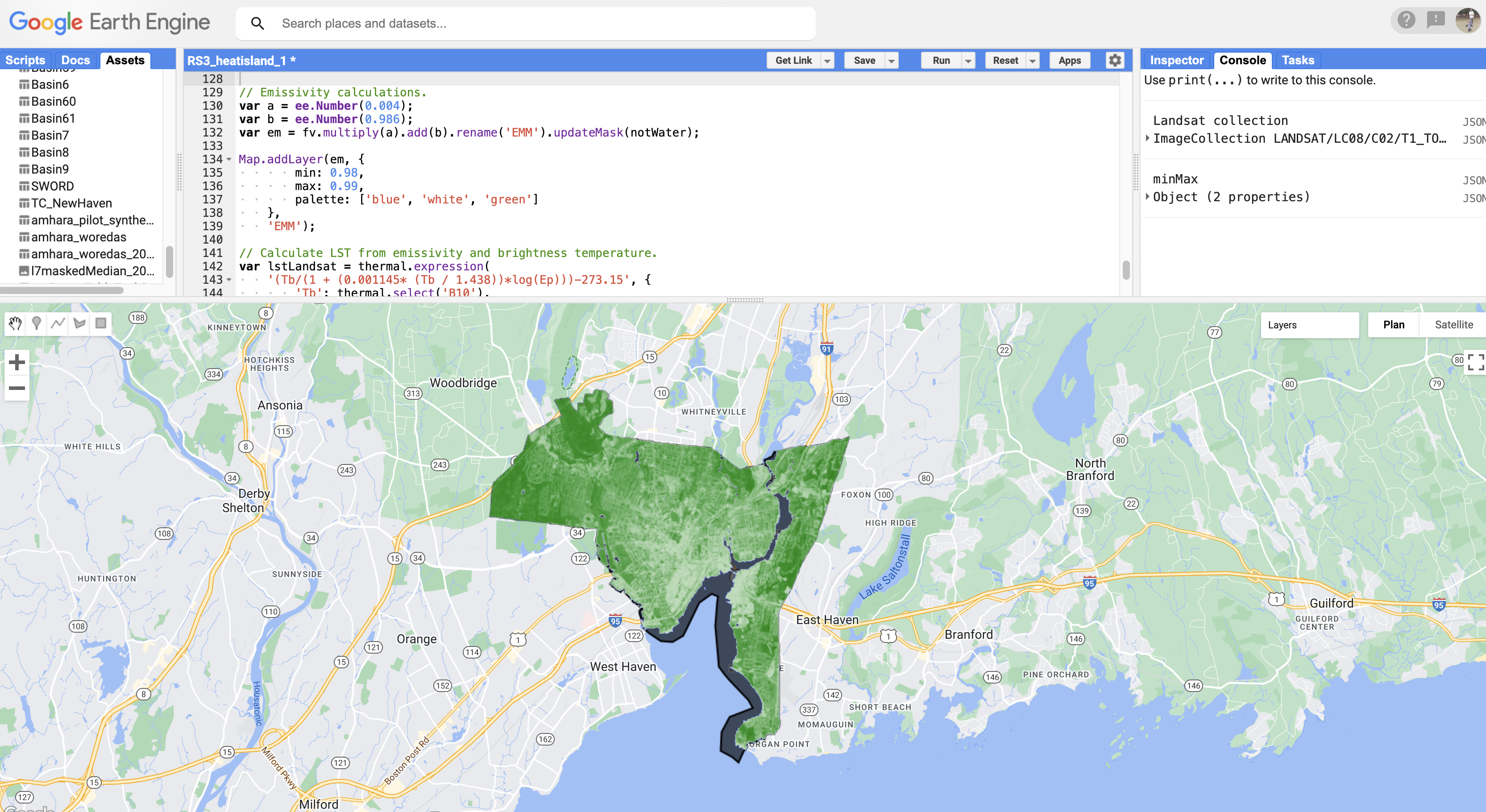
As seen in the figure, emissivity is lower over the built-up structures than over vegetation, which is expected. Note that different models of estimating emissivity would lead to differences in LST values and the SUHI intensity (Sekertekin and Bonafoni 2020, Chakraborty et al. 2021a).

Then, we combine this emissivity with the brightness temperature to calculate the LST for each pixel using a simple single-channel algorithm, which is a linearized approximation of the radiation transfer equation (Ermida et al. 2020).

// Calculate LST from emissivity and brightness temperature.
var lstLandsat = thermal.expression(
  '(Tb/(1 + (0.001145* (Tb / 1.438))*log(Ep)))-273.15', {
    'Tb': thermal.select('B10'),
    'Ep': em.select('EMM')
  }).updateMask(notWater);

Map.addLayer(lstLandsat, {
    min: 25,
    max: 35,
    palette: ['blue', 'white', 'red']
  },
  'LST_Landsat');

The Landsat-derived values correspond to those of the MODIS Terra daytime overpass. Overall, you do see similar patterns, but Landsat picks up a lot more heterogeneity than MODIS due to its finer resolution.