Defining Urban and Rural References

Now that we have estimates of LST using various products and algorithms, we can calculate the rural LST and subtract it from the urban LST to get the SUHI intensity. There are many ways to estimate the rural reference temperature (Li et al. 2022), and we will explore a few of them in this section.

The simplest and most commonly used method to get the rural reference when calculating the SUHI is to generate a buffered area around the urban boundary. The exact width of the buffer varies across studies, with buffers of 2–30 km in width being used in previous studies (Clinton and Gong 2013, Venter et al. 2021, Yao et al. 2019). In Earth Engine, generating such a buffer is simple:

// Function to subtract the original urban cluster from the buffered cluster to generate rural references.
function bufferSubtract(feature) {
  return ee.Feature(feature.geometry()
    .buffer(2000)
    .difference(feature.geometry()));
}

var ruralRef = regionInt.map(bufferSubtract);

Map.addLayer(ruralRef, {
    color: 'green'
  },
  'Buffer_ref');

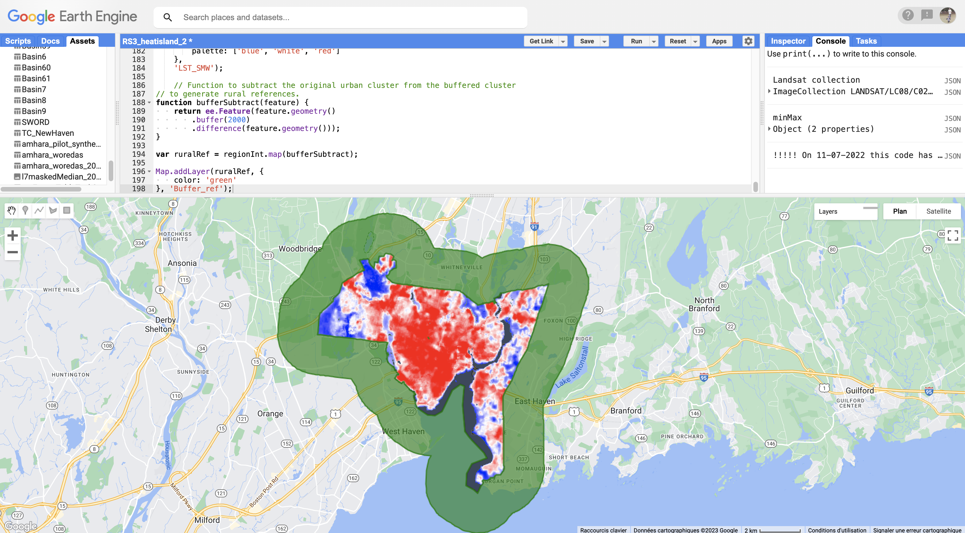
In the script above, a buffered polygon with a 2 km width is generated around the urban boundary, and the original urban boundary is subtracted from the buffered polygon.

Using a constant buffer assumes that all urban areas, regardless of size, have a similar influence around the city. This may be different for large cities. There is some evidence that there is a footprint of the SUHI that is dependent on the size of the city (Yang et al. 2019, Zhou et al. 2015). As such, another way to define the buffered region is to normalize its area by the area of the urban cluster it surrounds (Chakraborty et al. 2021b, Peng et al. 2011). An iterative method is one way to do so in Earth Engine. This method uses functions first to calculate buffers of different widths around a geometry and then select the buffered region that is closest in size to the original geometry.

// Define sequence of buffer widths to be tested.
var buffWidths = ee.List.sequence(30, 3000, 30);

// Function to generate standardized buffers (approximately comparable to area of urban cluster).
function bufferOptimize(feature) {
  function buff(buffLength) {
    var buffedPolygon = ee.Feature(feature.geometry()
      .buffer(ee.Number(buffLength)))
      .set({
        'Buffer_width': ee.Number(buffLength)
      });
    var area = buffedPolygon.geometry().difference(feature.geometry()).area();
    var diffFeature = ee.Feature(
      buffedPolygon.geometry().difference(feature.geometry()));
    return diffFeature.set({
      'Buffer_diff': area.subtract(feature.geometry().area()).abs(),
      'Buffer_area': area,
      'Buffer_width': buffedPolygon.get('Buffer_width')
    });
  }
  var buffed = ee.FeatureCollection(buffWidths.map(buff));
  var sortedByBuffer = buffed.sort({
    property: 'Buffer_diff'
  });
  var firstFeature = ee.Feature(sortedByBuffer.first());
  return firstFeature.set({
    'Urban_Area': feature.get('Area'),
    'Buffer_width': firstFeature.get('Buffer_width')
  });
}

// Map function over urban feature collection.
var ruralRefStd = regionInt.map(bufferOptimize);

Map.addLayer(ruralRefStd, {
    color: 'brown'
  },
  'Buffer_ref_std');

print('ruralRefStd', ruralRefStd);

Check the printed value on the Console. According to the result, within an uncertainty of 30 m, a buffer of 1170 m in width creates a polygon that is roughly equal to the area of the city. This function is best run via export when working with large feature collections.

The final way to define a rural reference does not use a buffer at all, but relies on land cover classes to select pixels that are urban versus non-urban (Chakraborty et al. 2020, Chakraborty and Lee 2019). For this, we will rely on the NLCD 2016 land cover data (Wickham et al. 2021) and create masks for urban and non-urban pixels.

// Select the NLCD land cover data.
var landCover = ee.Image('USGS/NLCD/NLCD2016').select('landcover');
var urban = landCover;

// Select urban pixels in image.
var urbanUrban = urban.updateMask(urban.eq(23).or(urban.eq(24)));

// Select background reference pixels in the image.
var nonUrbanVals = [41, 42, 43, 51, 52, 71, 72, 73, 74, 81, 82];
var nonUrbanPixels = urban.eq(ee.Image(nonUrbanVals)).reduce('max');
var urbanNonUrban = urban.updateMask(nonUrbanPixels);

Map.addLayer(urbanUrban.clip(regionInt), {
    palette: 'red'
  },
  'Urban pixels');
Map.addLayer(urbanNonUrban.clip(regionInt), {
    palette: 'blue'
  },
  'Non-urban pixels');

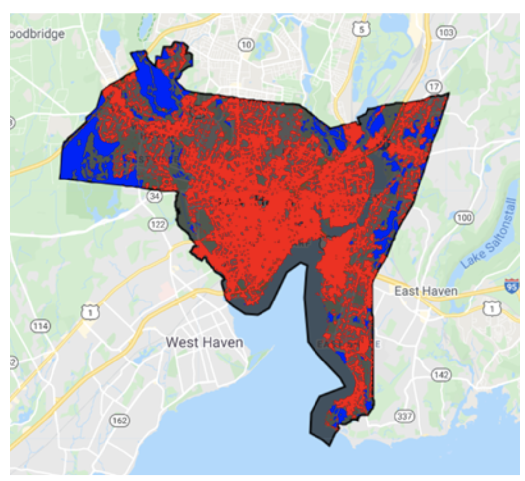
Subsequently, we can use these as masks to select urban versus rural LST pixels. You will find more about this in the next section.