Calculating the Surface Urban Heat Island Intensity

Since the SUHI is the temperature difference between the urban area and the rural reference, we will calculate summary temperature values for the urban boundary and the different versions of rural reference using the Landsat and MODIS LST.

// Define function to reduce regions and summarize pixel values to get mean LST for different cases.
function polygonMean(feature) {
  // Calculate spatial mean value of LST for each case making sure the pixel values are converted to °C from Kelvin.
  var reducedLstUrb = lstFinal.subtract(273.15).updateMask(notWater)
    .reduceRegion({
      reducer: ee.Reducer.mean(),
      geometry: feature.geometry(),
      scale: 30
    });
  var reducedLstUrbMask = lstFinal.subtract(273.15).updateMask(notWater)
    .updateMask(urbanUrban)
    .reduceRegion({
      reducer: ee.Reducer.mean(),
      geometry: feature.geometry(),
      scale: 30
    });
  var reducedLstUrbPix = lstFinal.subtract(273.15).updateMask(notWater)
    .updateMask(urbanUrban)
    .reduceRegion({
      reducer: ee.Reducer.mean(),
      geometry: feature.geometry(),
      scale: 500
    });
  var reducedLstLandsatUrbPix = landsatComp.updateMask(notWater)
    .updateMask(urbanUrban)
    .reduceRegion({
      reducer: ee.Reducer.mean(),
      geometry: feature.geometry(),
      scale: 30
    });
  var reducedLstRurPix = lstFinal.subtract(273.15).updateMask(notWater)
    .updateMask(urbanNonUrban)
    .reduceRegion({
      reducer: ee.Reducer.mean(),
      geometry: feature.geometry(),
      scale: 500
    });
  var reducedLstLandsatRurPix = landsatComp.updateMask(notWater)
    .updateMask(urbanNonUrban)
    .reduceRegion({
      reducer: ee.Reducer.mean(),
      geometry: feature.geometry(),
      scale: 30
    });
  // Return each feature with the summarized LSY values as properties.
  return feature.set({
    'MODIS_LST_urb': reducedLstUrb.get('LST_Day_1km'),
    'MODIS_LST_urb_mask': reducedLstUrbMask.get('LST_Day_1km'),
    'MODIS_LST_urb_pix': reducedLstUrbPix.get('LST_Day_1km'),
    'MODIS_LST_rur_pix': reducedLstRurPix.get('LST_Day_1km'),
    'Landsat_LST_urb_pix': reducedLstLandsatUrbPix.get('LST'),
    'Landsat_LST_rur_pix': reducedLstLandsatRurPix.get('LST')
  });
}

// Map the function over the urban boundary to get mean urban and rural LST for cases without any explicit buffer-based boundaries.
var reduced = regionInt.map(polygonMean);

As you know from the code above, we extract urban temperature from MODIS ('MODIS_LST_urb) and from Landsat and MODIS ('MODIS_LST_urb_pix' and 'Landsat_LST_urb_pix') after considering only the urban pixels within the boundary.

Corresponding values are also extracted from the rural reference (including using only rural reference pixels within the urban boundary). For the buffered regions (both using constant width and variable width), we define and call another function.

// Define a function to reduce region and summarize pixel values to get mean LST for different cases.
function refMean(feature) {
  // Calculate spatial mean value of LST for each case making sure the pixel values are converted to °C from Kelvin.
  var reducedLstRur = lstFinal.subtract(273.15).updateMask(notWater)
    .reduceRegion({
      reducer: ee.Reducer.mean(),
      geometry: feature.geometry(),
      scale: 30
    });
  var reducedLstRurMask = lstFinal.subtract(273.15).updateMask(notWater)
    .updateMask(urbanNonUrban)
    .reduceRegion({
      reducer: ee.Reducer.mean(),
      geometry: feature.geometry(),
      scale: 30
    });
  return feature.set({
    'MODIS_LST_rur': reducedLstRur.get('LST_Day_1km'),
    'MODIS_LST_rur_mask': reducedLstRurMask.get('LST_Day_1km')
  });
}

// Map the function over the constant buffer rural reference boundary one.
var reducedRural = ee.FeatureCollection(ruralRef).map(refMean);

// Map the function over the standardized rural reference boundary.
var reducedRuralStd = ruralRefStd.map(refMean);

print('reduced', reduced);
print('reducedRural', reducedRural);
print('reducedRuralStd', reducedRuralStd);

We can print the newly created feature collections to review these values for the different cases. Even though absolute MODIS and Landsat urban LSTs are different (29 for Landsat and 34 for MODIS), the SUHI is similar (3.6 C for MODIS and 4.8 C from Landsat). As one might expect, when only urban pixels are considered within the boundary, the average LST is higher (and lower for rural LST).

The SUHI variability within the city can then be displayed by subtracting the rural LST from the total LST:

// Display SUHI variability within the city.
var suhi = landsatComp
  .updateMask(urbanUrban)
  .subtract(ee.Number(ee.Feature(reduced.first()).get('Landsat_LST_rur_pix')));

Map.addLayer(suhi, {
    palette: ['blue', 'white', 'red'],
    min: 2,
    max: 8
  },
  'SUHI');

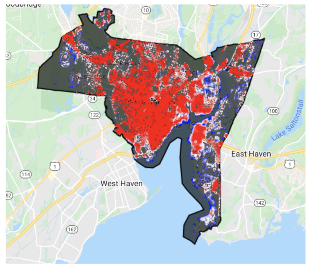
Spatial variability in SUHI for the period of interest for New Haven, Connecticut. Red pixels show higher values, and blue pixels show lower values.