How to Learn from This Guide
This page works best when you use it actively rather than reading it straight through. Preview the structure, answer questions from memory, and then return to the diagrams and notes to strengthen what you missed.
By the end, you should be able to...
- Explain GIS as a synthesis of theory, tools, and interpretive decision-making.
- Design an Earth Observation stack from data layer to user interface, including validation.
- Justify when to use supervised vs. unsupervised classification and why change detection needs pre-processing.
- Use spatial reasoning to connect proximity, clustering, and causality in scenario questions.
- Choose between satellite, drone, or fused workflows based on scale, detail, and logistics.
Recommended study cycle
- Preview: Scan headings, diagrams, and highlighted notes before reading paragraphs closely.
- Connect: Ask how each section links data, method, validation, and user need.
- Retrieve: Cover the page and answer a question in your own words before checking the model answer.
- Apply: Turn each concept into a short scenario: what problem, what sensor, what workflow, what limitation?
Core for the exam
Prioritize relationships and decisions: why a method fits a problem, how layers connect, and what must be validated.
How to use biographies
Treat named people as memory anchors for concepts, not as isolated facts to memorize.
What strong answers sound like
They identify the user need, choose a workflow, justify tradeoffs, and mention scientific or ethical limits.
Best retrieval habit
After each section, say the main idea aloud in two sentences. If you cannot, the section is not yet learned.
The Analytic Gaze
The contemporary landscape of Earth Observation (EO) and Geographic Information Science (GISc) is defined by a fundamental shift from static mapping to dynamic, multi-dimensional spatial intelligence. This evolution is necessitated by the compounding crises of climate change, urbanization, and ecological degradation, which require high-frequency, high-resolution monitoring systems that can transform raw pixel data into actionable knowledge. The geographer no longer merely records the world; they architect the systems that monitor its pulse.
Examination Protocol
The M3 T1-B examination is designed to test not only your retention of facts but your ability to synthesize disparate technologies into coherent solutions. Success requires a mastery of the "Functional Design" of space applications.
Exam Specifications
These 6 questions, totaling 20 points, are designed for the full 120-minute M3 T1-B examination. Questions contain multiple parts and cover the breadth of the course: cartography, GIS, remote sensing, image processing, AI/ML in EO, UI/UX, systems architecture, spatial analysis, and photogrammetry. Questions are scenario-based and require students to synthesize concepts from multiple lectures and workshops.
- Format: 6 Comprehensive Questions
- Weight: 20 Total Points
- Duration: 120 Minutes
- Nature: Scenario-based synthesis
The examination covers the full breadth of the Track 1-B curriculum. It is a 120-minute challenge where you must synthesize concepts from multiple lectures and workshops. The 6 questions below, totaling 20 points, are designed to evaluate your ability to think as a system architect, a spatial detective, and a digital artist.
Your answer routine for every scenario
1. Decode the verb
Design needs structure, justify needs reasons, and critique needs strengths plus weaknesses.
2. Name the workflow
State the problem, the user, the data source, the main method, and the output before adding detail.
3. Show the tradeoff
Explain why your chosen sensor, model, or interface is stronger than the alternatives for that case.
4. End with validation
Strong answers mention ground truth, HITL checks, uncertainty, ethics, or operational limits.
Thematic Roadmap: Core Competencies
| Pillar | Thematic Subject | Competency Focus | Primary Source Material |
|---|---|---|---|
| I | The AI Prompt Engineer | Technical Precision & Validation | AI/ML in EO (Mar 12), GEE Labs (Mar 17) |
| II | The GIS Synthesis | Theoretical & Interpretive Logic | Cartography (Feb 5), GISc (Feb 9), Geocoding (Feb 10), GIS as Art (M2 + May 5) |
| III | Earth Intelligence Systems | Systems Architecture & UI/UX | UI/UX (Mar 20), Web App Project (Mar 27), Image Processing (Mar 12) |
| IV | The Spatial Detective | Pattern Recognition & Causality | Spatial Analysis (Mar 6), John Snow Workshop (Mar 10), GISc (Feb 9) |
| V | Pixels to Knowledge | Classification & Spectral Analysis | Classification / Change Detection (Mar 12), RS eBook Ch. 6-7 |
| VI | Multi-Scale Sensing | Photogrammetry & Drone Logistics | Photogrammetry, Drone Assembly, SRTM/Elevation (May 5 + 7) |
🚨 Critical Pitfalls: The AI Prompt Engineer
When working with AI-driven EO workflows, technical precision is essential. Avoid these common mistakes:
- Vague Prompts: Failing to specify exact datasets (e.g., Landsat 8 vs. Sentinel-2).
- Missing Pre-processing: No mention of cloud masking, compositing, or scaling.
- No Output Specs: Failing to define the data format or visualization parameters.
🤖 The AI Revolution: Prompting and Foundation Models
Modern Earth Observation utilizes Large Language Models (LLMs) and Foundation Models pre-trained on massive unlabeled archives. These tools require a "Human in the Loop" (HITL) for validation and Chain-of-Thought (CoT) prompting for precision.
Chain-of-Thought (CoT)
Require the AI to explain its reasoning for a specific EO function choice. This allows you to audit the logic (e.g., verifying if the band assignment B4 for Red is correct for Landsat 8).
Foundation Models
Unlike traditional models that need thousands of labeled samples, Foundation Models provide a baseline of spatial understanding that can be fine-tuned for specific regions or tasks.
Key Professional Skill: No AI-generated workflow should be trusted until it has been confronted with reality. Use CoT to debug the pipeline and HITL to validate the thematic output against ground truth.
The Taxonomy of the Exam
Your performance is measured by how accurately you respond to the Command Verbs in each question. These verbs define the depth of the expected answer:
How Verbs Dictate Your Grade
In this exam, the verb is your grading rubric. If a question asks you to "Argue" and you only "Describe," you will not earn full points, no matter how accurate your facts are. "Argue" requires a position backed by evidence; "Justify" requires a rationale for a specific choice. Pay attention to the verbs. They tell you exactly what I expect.
DESIGN
Create a plan or specification showing the arrangement and workings of a system. Focus on flow and connectivity.
ARGUE
Provide reasons or evidence to support or oppose an idea. Requires logical proof, not just opinion.
JUSTIFY
Show adequate reason for a specific decision. Why this sensor? Why this algorithm?
CRITIQUE
Evaluate the strengths and weaknesses. A critique must be balanced and evidence-based.
EXPLAIN
Make a concept easy to understand. Focus on cause-and-effect and functional relationships.
COMPARE
Identify similarities and differences. Use a structured approach (e.g., spectral vs spatial resolution).
DESCRIBE
Give a factual account. Focus on the 'what' and 'how' of a topic or workflow.
WRITE
Compose professional text tailored to a specific audience (e.g., technical vs. policy-maker).
AI Prompt Engineering for Earth Observation
Modern AI systems (LLMs, vision-language models) can assist with tasks from data discovery to automated GEE script generation. However, the quality of AI output depends critically on the quality of the prompt you provide. Writing a precise, technically literate prompt is a professional skill.
Anatomy of an Effective GEE Prompt
A strong prompt is not vague; it reads like a technical specification. It must include all parameters the AI needs to generate a correct, runnable script.
| Component | What to Specify | Example |
|---|---|---|
| Dataset | Satellite collection and processing level | Landsat 8 Surface Reflectance (LANDSAT/LC08/C02/T1_L2) |
| Region & Time | Geographic bounding box and date range | Brazilian Amazon, -60 to -50 lon, -10 to -2 lat, 2019-2024 |
| Spectral Method | Vegetation index or classification method | NDVI using NIR (SR_B5) and Red (SR_B4); threshold > 0.6 = forest |
| Quality Controls | Cloud masking, compositing strategy | Cloud mask via QA_PIXEL band; dry-season median composite (Jun-Sep) |
| Output | Export format, resolution, visualization | Binary change map as GeoTIFF to Google Drive at 30m; red = deforestation |
| Extras | Area statistics, code comments | Calculate deforested area in km² using ee.Image.pixelArea(); add comments |
Human in the Loop: Why AI Output Must Be Validated
AI-generated code can be syntactically correct but logically flawed. Before trusting any AI output, verify:
1. Ground-Truth Validation
Compare AI-generated maps against validated datasets (Global Forest Watch, PRODES) or high-resolution imagery to check for false positives and false negatives.
2. Code Logic Inspection
Verify cloud masking is applied correctly, NDVI thresholds are appropriate for the biome, band assignments match the sensor, and the geographic extent is correct. LLMs may hallucinate GEE function names or use deprecated APIs.
The Architects of AI
If the pioneers of the past built the logic of space, the visionaries of the present are building the engines of intelligence. This contemporary "Lunch atop a Skyscraper" depicts the leaders who are currently forging the infrastructure of the Artificial Intelligence era.
How to study this section: treat it as an enrichment layer for the course. You do not need full biographies; instead, match each person to the role they represent in the intelligence stack: safety, hardware, scaling, scientific discovery, or human-centered design.

Contemporary Visionaries
In the 2025 "Person of the Year" selection, these individuals represent the diversity of thought (from hardware and safety to scaling laws and human-centered design) that characterizes the modern AI landscape.
Dario Amodei
Architect of AI safety. Championed "Constitutional AI" to align large language models with human values through guiding principles.
Daniella Amodei
Co-founder and President of Anthropic. Operationalized AI safety at scale, building the business infrastructure to ensure responsible deployment of frontier models.
Lisa Su
Hardware visionary. Transformed the compute ecosystem to provide the high-performance GPUs necessary for the AI revolution.
Elon Musk
Early advocate for AI safety and oversight. Founded xAI to pursue maximum truth-seeking and existential risk mitigation.
Jensen Huang
Architect of the Foundation. Pivoted the world to accelerated computing, turning the GPU into the engine of modern intelligence.
Sam Altman
The public face of generative AI. Orchestrated the global shift toward ubiquitous LLM tools and focused on the scaling laws of intelligence.
Demis Hassabis
Architect of AI for Science. Led the development of AlphaFold and other breakthroughs that apply AI to fundamental scientific discovery.
Yann LeCun
CNN Pioneer. Foundational architect of deep learning and vision systems; now advocating for world models and objective-driven AI.
Fei-Fei Li
The Architect of Data. Created ImageNet, unlocking deep learning's potential, and now leads the Human-Centered AI movement.
The Architects of Spatial Reasoning
Behind every pixel and polygon lies a legacy of intellectual bravery. These pioneers didn't just build tools; they invented new ways of seeing the world. They taught us that space is not just a container for objects, but a complex web of relationships that can be decoded, mapped, and mastered.
Use these as concept anchors: if you remember the idea attached to each name, you can retrieve the theory faster during the exam.

Dr. John Snow
The Spatial DetectiveThe father of modern epidemiology. By mapping the 1854 cholera outbreak in London, Snow proved that spatial analysis could solve medical mysteries and save lives.
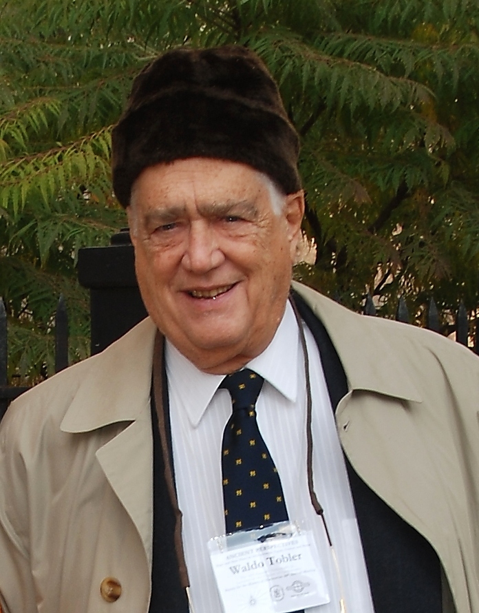
Waldo Tobler
The Analytical CartographerFormulated the First Law of Geography: "Everything is related to everything else, but near things are more related than distant things." His work laid the mathematical foundation for computational spatial science.

Jack Dangermond
The Infrastructure ArchitectFounder of Esri and a central figure in democratizing GIS. He transitioned mapping from specialized tools to a global infrastructure of spatial intelligence.
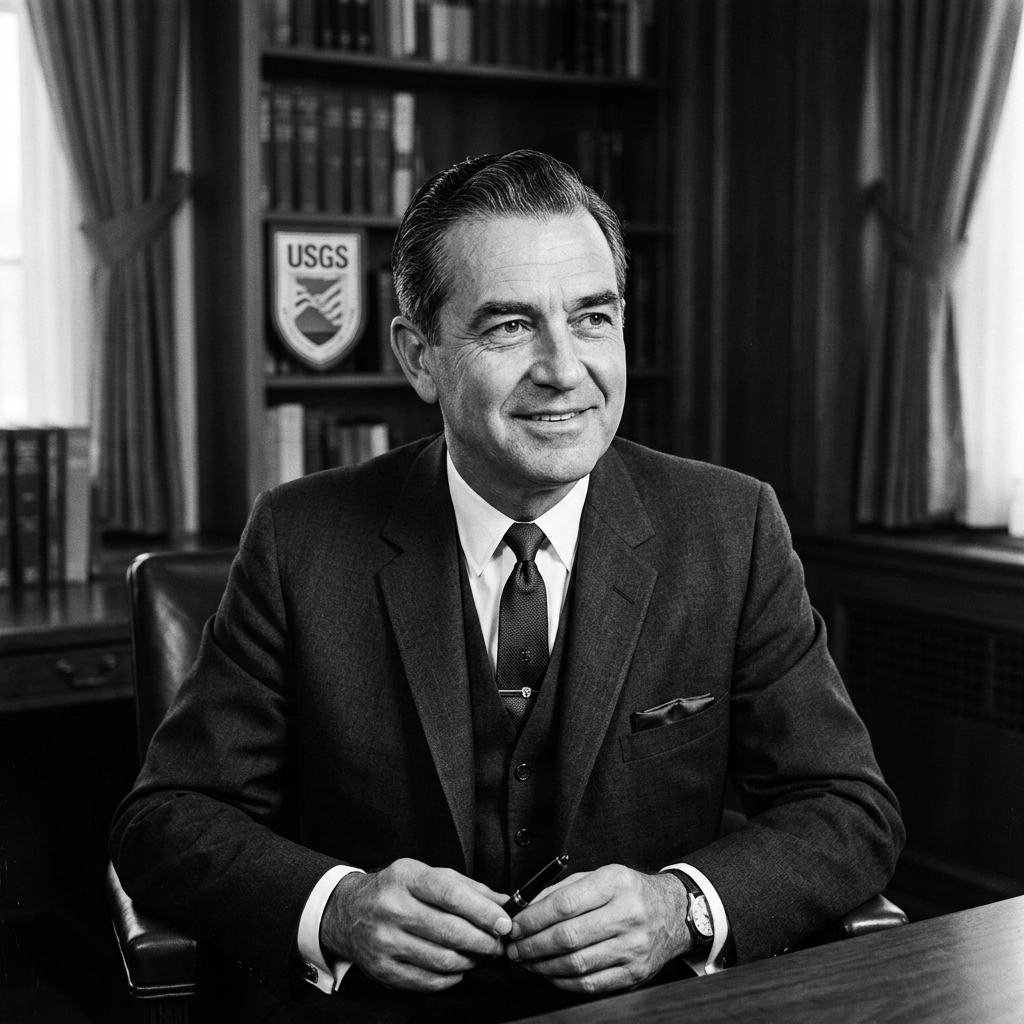
William T. Pecora
The Father of LandsatA pioneer of Earth observation and the visionary behind the Landsat program. During his tenure at USGS, Pecora championed the civilian satellite system that became the longest-running EO program in history.
Summary of Big Ideas
Spatial Reasoning
The ability to use geography to solve problems, recognize patterns, and understand the logic of proximity and location.
Functional Design
Architecting space applications that prioritize user needs, clear workflows, and decoupled tiers for resilience.
GeoAI Synthesis
The convergence of spatial science and artificial intelligence, amplifying the analyst's capacity for planetary-scale monitoring.
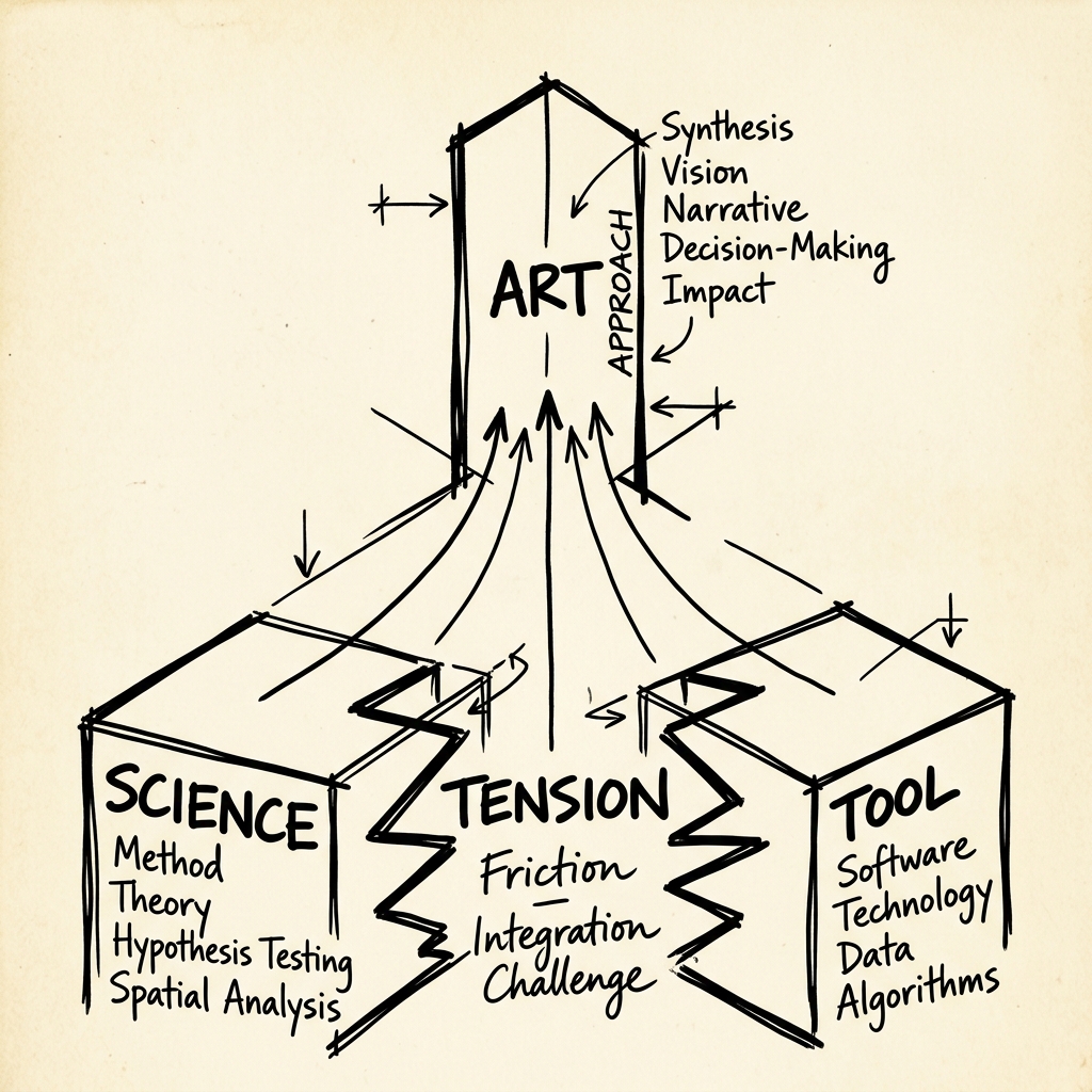
The GIS Synthesis
Geographic Information Systems (GIS) represent more than a simple intersection; they are a site of productive tension. We recognize an inherent "battle" between Science (the academic theory and spatial ontology) and the Tool (the mechanical execution and software mechanics). In reality, these are synthesized into the Approach, which is the true Art of the geographer. To master GIS is to wield the approach that resolves this tension, turning raw theory and cold tools into meaningful spatial wisdom.
Epistemological Status: The GIS Triad
Dr. Sounny posits a tripartite perspective that reconciles the functional utility of the technology with its scientific depth and artistic subjectivity. Understanding GIS as a Tool, a Science, and an Art is the foundation of professional spatial reasoning.
| Paradigm | Focus Area | Scientific Inquiry | Implementation |
|---|---|---|---|
| GIS as Tool | Functionality | Operational efficiency; geocoding mechanics. | Routine workflows; batch processing. |
| GIS as Science | Representation | Spatial laws (Tobler); MAUP; Uncertainty. | Ontology of place; spatial reasoning. |
| GIS as Art | Interpretation | Subjective visualization; cartographic narratives. | Hillshade azimuths; band combinations. |
Architectural Integrity
A robust space application is built on a decoupled, tiered architecture. The Data Layer ingests raw telemetry and spectral bands. The Back-end Logic performs radiometric normalization and index calculation. The Front-end mediates the human-data interface through progressive disclosure. Understanding this flow is essential for designing resilient environmental monitoring systems.
The Emerging Fourth Tier: The Intelligence Layer
The traditional three-tier stack is evolving. A new Intelligence Layer is emerging between the Front-end (UX) and the Back-end (Logic). Rather than requiring the user to understand how to formulate queries, select datasets, or invoke processing pipelines manually, an AI agent sits between the interface and the system's logic, mediating the entire workflow: interpreting natural language requests, selecting appropriate datasets from the Data Layer, orchestrating processing in the Back-end, and delivering results to the Front-end for visualization.
This concept is being actively explored in student research. TerraXsite.com, a project by MSS student Assaf Shaked, investigates how this fourth tier adds value by serving as an intelligent intermediary between the user and all parts of the stack, amplifying the analyst's capabilities without requiring deep technical knowledge of each layer.
Think of the Intelligence Layer as the difference between manually writing SQL queries against PostGIS, versus describing your analysis goal in plain language and having an AI agent construct, execute, and visualize the query for you.
Mastering the Diagram
When you architect a stack, do not just list components; draw the relationships. A strong system diagram includes:
- Clear Tiers: Visible separation between Cloud, Server, and Client.
- Data Flow: Arrows showing raw imagery becoming actionable alerts.
- Functional Labels: Identifying specific bands (e.g., TIRS Band 10) and libraries (e.g., Leaflet.js).
- UI Context: Sketching where the map and controls live.
The Spatial Detective
Spatial analysis is fundamentally an act of detective work. It requires identifying patterns, investigating anomalies, and establishing causality across geographic space. Whether tracking a virus like John Snow or monitoring deforestation in the Amazon, the spatial detective uses the layers of the Earth to reveal hidden truths.
Case Study: The Broad Street Pump
To understand the 'Analytical Gaze', we look back at the origins of spatial reasoning. Below is John Snow's original Ghost Map of the 1854 cholera outbreak in London. The clustering of deaths around the Broad Street pump demonstrates the Kernel Density Estimation (KDE) principle we use today in GeoAI to detect hotspots from point data.
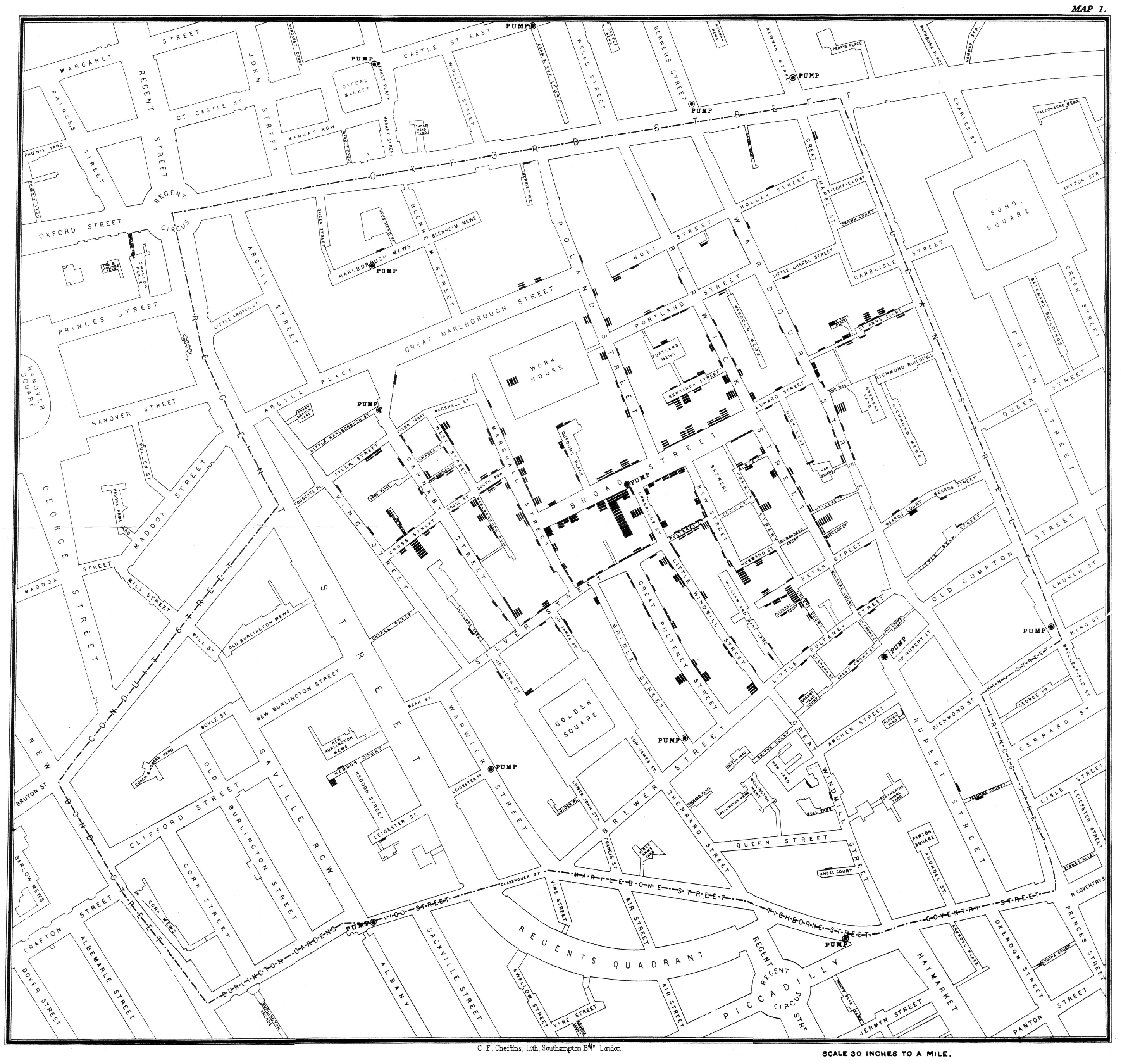
John Snow's Ghost Map (1854): Each bar represents a cholera death. The clustering around the Broad Street pump provided the spatial evidence that contaminated water was the source.

"To be a spatial detective is to understand that every point has a story, and every map is a witness. We don't just find where things are; we discover why they belong there."
Ill-Structured Scenario: The Regional Decision
The Scenario: You are the lead analyst for a reforestation project in an undisclosed tropical region. You must choose a specific study area (A, B, or C) based solely on its spectral suitability and temporal continuity. Region A has consistent Landsat 8 coverage but high cloud frequency (80%). Region B has Sentinel-2 coverage but suffers from high radiometric noise. Region C is a conflict zone where field validation is impossible.
Decision 1: Workflow Choice
In Region C, would you justify a Supervised or Unsupervised classification workflow?
Decision 2: Mitigation
In Region A, what specific pre-processing step is mandatory to retrieve actionable NDVI despite the cloud cover?
A synthesis answer: For Decision 1, choose Unsupervised Classification for Region C because the lack of field access makes reliable training data collection impossible. For Decision 2, mandatory pre-processing in Region A involves Median Compositing and Cloud Masking using the QA_PIXEL band. The critique of Region A is that while spectral quality is high, the high cloud frequency may hide the specific 5-year change signal unless multiple years are fused.
The John Snow Method: From Points to Proof
In the John Snow workshop, you recreated one of history's most famous spatial analyses. Understanding the specific technique and the theory behind it is essential.
Kernel Density Estimation (KDE)
The technique you used in the workshop to identify the contamination source. KDE creates a continuous "heat surface" from discrete point locations (cholera deaths), revealing spatial clustering. The peak of the density surface pointed directly to the Broad Street pump.
Also relevant: Voronoi (Thiessen) Polygons can define pump "service areas," showing which residents would naturally draw water from each pump.
Tobler's Law in Action
"Near things are more related than distant things." Snow's hypothesis relied on this principle: people living closer to the contaminated pump were more likely to drink from it, and therefore more likely to become ill.
The spatial decay of death frequency with distance from the Broad Street pump directly demonstrates Tobler's First Law. Proximity was the mechanism of causation.
Ethical Stewardship Checklist
As a spatial detective, you must navigate the ethical pitfalls inherent in geographic inquiry. Before publishing any spatial analysis, verify your compliance with these principles:
Spatial Privacy & De-anonymization
Can individual identities be reconstructed from movement trajectories or location patterns? Implement differential privacy or spatial aggregation to protect subjects.
Modifiable Areal Unit Problem (MAUP)
Are your results artifacts of the boundaries you chose? Always test findings at multiple scales (e.g., zip code vs. census tract) to ensure consistency.
Ecological Fallacy
Avoid assuming that individual members of a group possess the average characteristics of that group. Spatial averages mask local variation and individual nuance.
Algorithmic Equity
Does your data source (e.g., mobile data) under-represent specific demographics? Acknowledge coverage gaps and their impact on policy recommendations.
Pixels to Knowledge
The analytical pipeline of Earth Observation transforms raw satellite pixels into actionable knowledge. This section covers the two critical stages of that pipeline: classifying what the sensor sees, and detecting how the landscape has changed over time. Mastering these concepts requires understanding both the methods and the essential pre-processing that makes them reliable.
Pixels to Knowledge Pipeline
1. Image Classification
2. Change Detection
Image Classification: Philosophical Comparison
Classification assigns a thematic label (forest, water, urban) to every pixel in an image based on its spectral signature. Choosing the right philosophy is the first step in any remote sensing workflow.
| Feature | Supervised Classification | Unsupervised Classification |
|---|---|---|
| Requirement | Prior knowledge and training samples. | No prior knowledge; auto-clustering. |
| Analyst Role | Defines classes and selects training pixels. | Assigns thematic meaning to clusters post-hoc. |
| Best For... | Precise mapping of known target classes. | Exploring data or classifying remote areas. |
| Validation | Accuracy assessment via Confusion Matrix. | Post-hoc interpretation and verification. |
Validation Metrics: Accuracy & Chance
After classification, accuracy is assessed using two gold-standard metrics:
- Confusion Matrix: A cross-tabulation of predicted classes versus ground truth (Reference) pixels.
- Kappa Coefficient: A statistical measure that accounts for the accuracy occurring by random chance. Kappa > 0.8 indicates excellent agreement.
Change Detection: Mandatory Pre-processing
Change detection compares satellite images from different dates. However, raw spectral values are influenced by atmosphere and geometry. The following pre-processing steps are mandatory for scientific validity.
| Workflow Step | The Technical Necessity | The Penalty of Omission |
|---|---|---|
| Atmospheric Correction | Converts Top-of-Atmosphere (TOA) Digital Numbers to Surface Reflectance. | Haze, clouds, and sun angle create false "changes" in pixel values. |
| Geometric Co-registration | Aligns pixel (x,y) in T1 to exactly the same ground location in T2. | Pixel shifts cause feature edges (roads, buildings) to appear as change. |
| Radiometric Normalization | Ensures sensors from different dates or platforms share a common scale. | Inconsistent brightness levels prevent quantitative comparison. |
Scientific Credibility
Without these steps, your algorithm detects sensor artifacts rather than landscape change. This leads to erroneous reports on deforestation or urban growth. Pre-processing is the bridge between raw data and legitimate science.
🛰️ Satellite Band Cheat Sheet
A quick-reference for the three workhorses of Earth Observation. Know your sensor, know your bands, know your mission timeline.
Mission Timeline & Operational Status
| Mission | Launch Date | Status | Spatial Res. | Revisit | Operator |
|---|---|---|---|---|---|
| LANDSAT PROGRAM (USGS / NASA) | |||||
| Landsat 1 (ERTS-1) | Jul 23, 1972 | Decommissioned (1978) | 80 m (MSS) | 18 days | USGS/NASA |
| Landsat 2 | Jan 22, 1975 | Decommissioned (1982) | 80 m (MSS) | 18 days | USGS/NASA |
| Landsat 3 | Mar 5, 1978 | Decommissioned (1983) | 80 m (MSS) | 18 days | USGS/NASA |
| Landsat 4 | Jul 16, 1982 | Decommissioned (1993) | 30 m (TM) | 16 days | USGS/NASA |
| Landsat 5 | Mar 1, 1984 | Decommissioned (2013) | 30 m (TM) | 16 days | USGS/NASA |
| Landsat 6 | Oct 5, 1993 | Launch Failure | N/A | N/A | USGS/NASA |
| Landsat 7 | Apr 15, 1999 | Operational (degraded SLC) | 30 m (ETM+), 15 m pan | 16 days | USGS/NASA |
| Landsat 8 | Feb 11, 2013 | ✓ Operational | 30 m (OLI), 15 m pan | 16 days | USGS/NASA |
| Landsat 9 | Sep 27, 2021 | ✓ Operational | 30 m (OLI-2), 15 m pan | 16 days | USGS/NASA |
| COPERNICUS SENTINEL-2 (ESA) | |||||
| Sentinel-2A | Jun 23, 2015 | ✓ Operational | 10 / 20 / 60 m (MSI) | 10 days (single) | ESA |
| Sentinel-2B | Mar 7, 2017 | ✓ Operational | 10 / 20 / 60 m (MSI) | 5 days (combined) | ESA |
| Sentinel-2C | Sep 5, 2024 | ✓ Commissioning | 10 / 20 / 60 m (MSI) | 5 days (combined) | ESA |
| MODIS (NASA) | |||||
| MODIS (Terra) | Dec 18, 1999 | ✓ Operational | 250 / 500 / 1000 m | 1-2 days | NASA |
| MODIS (Aqua) | May 4, 2002 | ✓ Operational | 250 / 500 / 1000 m | 1-2 days | NASA |
Landsat 8/9 OLI Band Designations
| Band | Name | Wavelength (μm) | Resolution | Primary Application |
|---|---|---|---|---|
| B1 | Coastal Aerosol | 0.43 - 0.45 | 30 m | Coastal water, aerosol studies |
| B2 | Blue | 0.45 - 0.51 | 30 m | Bathymetry, soil/vegetation distinction |
| B3 | Green | 0.53 - 0.59 | 30 m | Vegetation vigor (peak reflectance) |
| B4 | Red | 0.64 - 0.67 | 30 m | Vegetation discrimination, NDVI |
| B5 | NIR | 0.85 - 0.88 | 30 m | Biomass, shoreline mapping, NDVI |
| B6 | SWIR 1 | 1.57 - 1.65 | 30 m | Soil moisture, snow/ice differentiation |
| B7 | SWIR 2 | 2.11 - 2.29 | 30 m | Mineral mapping, soil moisture |
| B8 | Panchromatic | 0.50 - 0.68 | 15 m | Image sharpening (pan-sharpening) |
| B9 | Cirrus | 1.36 - 1.38 | 30 m | Cirrus cloud detection |
| B10 | TIRS 1 (Thermal) | 10.6 - 11.19 | 100 m | Surface temperature, urban heat islands |
| B11 | TIRS 2 (Thermal) | 11.5 - 12.51 | 100 m | Surface temperature (improved accuracy) |
Sentinel-2 MSI Band Designations
| Band | Name | Wavelength (μm) | Resolution | Primary Application |
|---|---|---|---|---|
| B1 | Coastal Aerosol | 0.443 | 60 m | Aerosol detection, atmospheric correction |
| B2 | Blue | 0.490 | 10 m | Water body mapping, soil/vegetation |
| B3 | Green | 0.560 | 10 m | Vegetation peak reflectance |
| B4 | Red | 0.665 | 10 m | Vegetation classification, NDVI |
| B5 | Red Edge 1 | 0.705 | 20 m | Vegetation stress, chlorophyll content |
| B6 | Red Edge 2 | 0.740 | 20 m | Vegetation health, leaf area index |
| B7 | Red Edge 3 | 0.783 | 20 m | Vegetation canopy water content |
| B8 | NIR | 0.842 | 10 m | Biomass, NDVI, land/water boundary |
| B8A | NIR Narrow | 0.865 | 20 m | Refined vegetation analysis |
| B9 | Water Vapour | 0.945 | 60 m | Atmospheric water vapour estimation |
| B10 | SWIR (Cirrus) | 1.375 | 60 m | Cirrus cloud detection |
| B11 | SWIR 1 | 1.610 | 20 m | Snow/ice, moisture, burn scars |
| B12 | SWIR 2 | 2.190 | 20 m | Geology, mineral content, soil |
MODIS Key Bands (36 Total, Selected for EO)
| Band | Name | Wavelength (μm) | Resolution | Primary Application |
|---|---|---|---|---|
| B1 | Red | 0.620 - 0.670 | 250 m | Land/cloud boundaries, NDVI |
| B2 | NIR | 0.841 - 0.876 | 250 m | Vegetation, NDVI, land/cloud |
| B3 | Blue | 0.459 - 0.479 | 500 m | Soil/vegetation, ocean color |
| B4 | Green | 0.545 - 0.565 | 500 m | Vegetation vigor, ocean color |
| B6 | SWIR 1 | 1.628 - 1.652 | 500 m | Snow/cloud discrimination |
| B7 | SWIR 2 | 2.105 - 2.155 | 500 m | Snow/ice, land properties |
| B20 | Thermal | 3.660 - 3.840 | 1000 m | Sea surface temperature, fire detection |
| B31 | Thermal IR | 10.780 - 11.280 | 1000 m | Land surface temperature, clouds |
| B32 | Thermal IR | 11.770 - 12.270 | 1000 m | Surface/cloud temperature |
Key Insight: The Resolution Tradeoff
Notice the inverse relationship between spatial resolution and temporal resolution. Landsat (30 m, 16-day revisit) provides fine spatial detail but infrequent coverage. MODIS (250-1000 m, daily revisit) sacrifices spatial precision for near-continuous global monitoring. Sentinel-2 (10 m, 5-day revisit) represents the current "sweet spot" for operational land monitoring. Choosing the right sensor depends on whether your application prioritizes spatial detail or temporal frequency.
From Satellites to Drones
The final frontier of Earth Observation integrates orbital sensors with near-surface platforms. Understanding when to use each, and how to combine them, is the mark of a complete spatial analyst. This section covers the fundamental comparison between radar-based satellite elevation and optical drone photogrammetry.
Elevation Modeling: Two Approaches
| Feature | SRTM (Satellite Radar) | Drone Photogrammetry (SfM) |
|---|---|---|
| Sensor Type | Active (Radar, InSAR) | Passive (Optical Camera) |
| Spatial Resolution | ~30m globally | 1-10 cm (centimeter-level) |
| Coverage | Near-global, single acquisition | Small area per flight (limited battery) |
| Primary Output | DSM (radar reflects off canopy and rooftops) | DSM initially; can be filtered to DEM with ground classification |
DSM vs. DEM: Why It Matters
A Digital Surface Model (DSM) includes the tops of trees, buildings, and all surface features. A Digital Elevation Model (DEM) represents the bare earth. The distinction is critical: hydrological modeling (water flow) requires a DEM, while urban planning (building height analysis) requires a DSM. Using the wrong model produces incorrect results.
Data Fusion: Why Neither Alone Is Sufficient
Consider monitoring coastal erosion along a 50 km stretch of coastline. Neither satellite data nor drone data alone can solve this problem optimally.
Satellite Contribution
Sentinel-2 or Landsat provides wide-area coverage of the entire 50 km coastline at regular intervals (every 5-16 days). This gives temporal frequency and the ability to detect broad erosion trends over years.
Limitation: 10-30m resolution cannot resolve individual cliff collapses or small landslides.
Drone Contribution
Drones provide ultra-high-resolution detail (cm-level) at specific hotspot locations identified from the satellite time series. They capture detailed 3D point clouds of cliff faces and beach profiles.
Limitation: Cannot realistically cover 50 km consistently (battery life, flight regulations).
"The satellite data identifies where to look; the drone data tells you how bad it is. Together, they form a multi-scale observation system that neither can achieve alone."
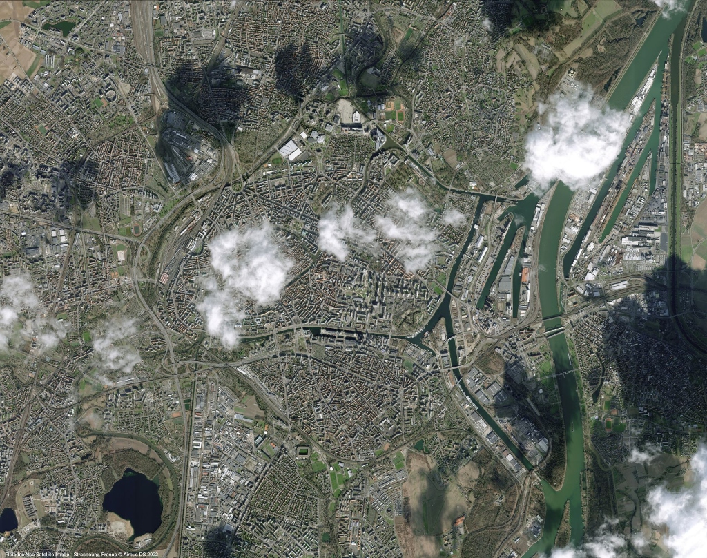
Georeferencing & Coordinate Reference Systems
Every spatial dataset must be anchored to the Earth's surface. Georeferencing is the process of assigning real-world coordinates to raster data (such as scanned maps or unreferenced imagery) using Ground Control Points (GCPs). The quality of every downstream analysis depends on the accuracy of this foundational step.
Coordinate Reference Systems (CRS)
A CRS defines how 2D map coordinates relate to real locations on the Earth. Every spatial project must declare its CRS. Mismatched CRS between layers is the most common source of spatial error.
Geographic CRS (GCS)
Uses latitude and longitude (degrees) on a 3D ellipsoid. Example: WGS 84 (EPSG:4326), the standard for GPS and most global datasets.
Projected CRS (PCS)
Transforms 3D coordinates onto a flat 2D surface using mathematical projections. Example: UTM Zone 32N (EPSG:32632), used for Strasbourg-area mapping with units in meters.
| Concept | Definition | Why It Matters |
|---|---|---|
| Datum | A mathematical model of the Earth's shape (ellipsoid + reference point). | WGS 84 is the global standard; local datums (e.g., ED50) may shift positions by tens of meters. |
| Projection | The method for flattening 3D coordinates onto a 2D map. | All projections distort either area, shape, distance, or direction. Choose based on the analysis goal. |
| Ground Control Points | Known locations used to anchor raster imagery to real-world coordinates. | More GCPs (well-distributed) yield lower RMS error and more accurate georeferencing. |
| RMS Error | Root Mean Square Error, measuring the average residual after transformation. | Lower RMS indicates better alignment. Target: less than 1 pixel for precise work. |
| On-the-Fly (OTF) Projection | GIS software temporarily reprojects layers to match the map view CRS. | Enables visual overlay of mixed-CRS data without permanently altering coordinates. |
Geocoding: From Addresses to Coordinates
Geocoding is the process of converting human-readable addresses (e.g., "1 Illkirch-Graffenstaden, France") into geographic coordinates (latitude, longitude). Reverse geocoding does the opposite: converting coordinates into a readable address. This is a core GIS operation that underpins location-based services, logistics, and spatial epidemiology.
Batch Geocoding
Processing many addresses at once using APIs (e.g., Nominatim, Google Geocoding API) or GIS tools (QGIS MMQGIS plugin). Essential for datasets with hundreds or thousands of location entries.
Workshop skill: You performed batch geocoding using the MMQGIS plugin in QGIS, converting CSV address lists into point layers.
Address Validation
Not all addresses geocode successfully. Common issues: ambiguous place names, missing postal codes, non-standardized formats. Always check the match rate and visually inspect outliers on the map.
Quality check: A point geocoded to (0, 0) typically indicates a failed match, not a location in the Gulf of Guinea.
Linear Geocoding
Assumes addresses vary linearly along a street centerline. The geolocator estimates a point's position by interpolating between known start and end address ranges (e.g., the 100-200 block of Easy Street).
Tradeoff: Lightweight and often free, but assumes equal spacing and sequential ordering, which may not reflect reality.
Area (Areal) Geocoding
Uses building footprint polygons, each tagged with a street number. The geolocator searches for a matching polygon and returns its centroid. Does not assume spacing or ordering.
Tradeoff: More accurate than linear geocoding, but significantly more data-intensive and computationally expensive.
Spectral Indices & Vegetation Analysis
Spectral indices are mathematical combinations of spectral bands that highlight specific surface properties. They compress multi-band imagery into single-value layers optimized for a particular analysis objective. Knowing which index to apply, and which bands it uses, is a core remote sensing competency.
| Index | Formula | Bands (Landsat 8) | Application |
|---|---|---|---|
| NDVI | (NIR - Red) / (NIR + Red) | B5, B4 | Vegetation health and density. Values range from -1 to +1; healthy vegetation > 0.3. |
| NDWI | (Green - NIR) / (Green + NIR) | B3, B5 | Water body detection. Positive values indicate open water surfaces. |
| NDBI | (SWIR - NIR) / (SWIR + NIR) | B6, B5 | Built-up / urban area mapping. Higher values suggest impervious surfaces. |
| EVI | 2.5 * (NIR - Red) / (NIR + 6*Red - 7.5*Blue + 1) | B5, B4, B2 | Enhanced vegetation index; more robust in high-biomass areas than NDVI. |
| NBR | (NIR - SWIR2) / (NIR + SWIR2) | B5, B7 | Burn severity mapping. dNBR (pre-fire minus post-fire) quantifies fire impact. |
Why NDVI Works
Healthy vegetation absorbs red light for photosynthesis and strongly reflects near-infrared (NIR) light due to cellular structure. The ratio exploits this contrast: high NDVI means the plant is actively photosynthesizing. Stressed or dead vegetation reflects more red and less NIR, producing lower NDVI values. This principle applies across all optical sensors.
Hyperspectral Remote Sensing
While multispectral sensors (Landsat, Sentinel-2) capture data in broad spectral bands (typically 4 to 13), hyperspectral sensors record hundreds of narrow, contiguous bands across the electromagnetic spectrum. This enables precise material identification based on diagnostic spectral absorption features.
Key Characteristics
- Band count: Typically 100 to 400+ narrow bands (10-20 nm wide).
- Spectral libraries: Reference spectra (e.g., USGS Spectral Library) used for matching.
- Curse of dimensionality: Hundreds of bands require dimensionality reduction (PCA) before classification.
- Data volume: Much larger files than multispectral, requiring specialized processing.
Applications
- Mineral mapping: Identifying specific rock types and ore deposits.
- Precision agriculture: Detecting plant stress before visible symptoms appear.
- Water quality: Measuring chlorophyll-a concentration and algal blooms.
- Atmospheric correction: Deriving water vapor content for calibrating other sensors.
Radar Remote Sensing & Terrain Mapping
Unlike optical sensors that rely on reflected sunlight, Synthetic Aperture Radar (SAR) is an active sensor that transmits its own microwave pulses and measures the backscattered signal. This makes SAR weather-independent and capable of imaging day or night, penetrating cloud cover that blocks optical observation.
| Feature | Optical (Passive) | SAR (Active) |
|---|---|---|
| Energy source | Reflected sunlight | Self-generated microwave pulses |
| Cloud penetration | Blocked by clouds | Penetrates clouds, rain, smoke |
| Day/night | Daytime only | Day and night |
| Measured property | Surface reflectance (spectral) | Surface roughness, moisture, structure |
| Key platforms | Landsat, Sentinel-2, MODIS | Sentinel-1, ALOS PALSAR, TerraSAR-X |
InSAR (Interferometric SAR)
Compares the phase difference between two SAR acquisitions of the same area taken at different times. Phase shifts reveal millimeter-scale surface deformation, enabling monitoring of land subsidence, volcanic uplift, glacier movement, and earthquake damage.
SAR Polarization
SAR transmits and receives in different polarization modes (HH, VV, HV, VH). Co-polarized (HH, VV) is sensitive to surface roughness. Cross-polarized (HV, VH) is sensitive to volume scattering (e.g., forest canopy structure), making it valuable for biomass estimation.
Global Monitoring & Climate Applications
Earth Observation underpins global environmental monitoring by providing consistent, repeatable measurements of the planet's atmosphere, land surface, and oceans. Understanding how EO data feeds into climate policy and the Sustainable Development Goals (SDGs) bridges the gap between technical remote sensing and real-world decision-making.
Essential Climate Variables (ECVs)
- Land Surface Temperature (LST): Measured via thermal infrared (Landsat TIRS, MODIS); critical for UHI monitoring.
- Sea Surface Temperature (SST): Tracked by MODIS and VIIRS for ocean circulation and El Nino/La Nina patterns.
- Ice extent: Arctic/Antarctic monitoring using SAR (Sentinel-1) and passive microwave sensors.
- Atmospheric CO2: Measured by OCO-2 satellite, validating emission inventories.
EO for SDGs
- SDG 11 (Sustainable Cities): Urban sprawl mapping via classification time series.
- SDG 13 (Climate Action): Fire severity (dNBR), deforestation alerts (GLAD/Hansen).
- SDG 14 (Life Below Water): Coral reef health and ocean color monitoring (Sentinel-3 OLCI).
- SDG 15 (Life on Land): Forest cover change, NDVI anomaly detection for drought early warning.
Copernicus Services
The EU Copernicus programme provides six thematic services: Land, Marine, Atmosphere, Climate Change, Security, and Emergency Management. Each transforms raw Sentinel satellite data into ready-to-use products. The Copernicus Emergency Management Service (CEMS) provides rapid mapping within hours of a natural disaster, supporting civil protection agencies.
Google Earth Engine: Practical Workflows
Google Earth Engine (GEE) is a cloud-based geospatial analysis platform that provides access to petabytes of satellite imagery and a JavaScript/Python API for large-scale computation. Mastering GEE workflows means understanding the key operations: data selection, filtering, compositing, index calculation, and export.
Core GEE Concepts
ImageCollection
A stack of images (e.g., all Landsat 8 scenes). You filter by date, bounds, and cloud cover to select relevant scenes, then reduce (e.g., median composite) to collapse the stack into a single cloud-free image.
Server-side vs. Client-side
GEE processes data on Google's servers (server-side). ee.Number, ee.Image are server objects. Use .getInfo() sparingly to bring results client-side, as it blocks execution.
Standard GEE Workflow Pattern
- Define Area of Interest (AOI): Use
ee.Geometryor draw directly on the map. - Select Collection: Choose the appropriate dataset (e.g.,
'LANDSAT/LC08/C02/T1_L2'for Landsat 8 Level-2). - Filter:
.filterDate(),.filterBounds(aoi),.filter(ee.Filter.lt('CLOUD_COVER', 20)). - Pre-process: Apply scaling factors, cloud masking (QA_PIXEL band), and atmospheric correction.
- Compute: Calculate indices (NDVI, NDWI), perform classification, or generate composites using
.median(). - Visualize: Use
Map.addLayer()with visualization parameters (min, max, palette). - Export:
Export.image.toDrive()to save results as GeoTIFF for use in QGIS or other tools.
Active Recall Studio
Try to answer each question out loud before revealing the model response. If your answer is vague, return to the section and tighten it until you can explain the idea in one or two precise sentences.
Last-minute self-check
- I can explain why Google Maps is not enough for scientific Earth Observation.
- I can compare supervised and unsupervised classification without mixing up their inputs.
- I can draw a multi-tier EO system and label what happens in each layer.
- I can connect Tobler's Law to a real example of spatial clustering or causality.
- I can distinguish DSM from DEM and explain why the choice matters for analysis.
Reference Library
The following resources are essential for advanced study and practical application development within the ISU curriculum.