The Grand Canyon: A Window into Earth's History
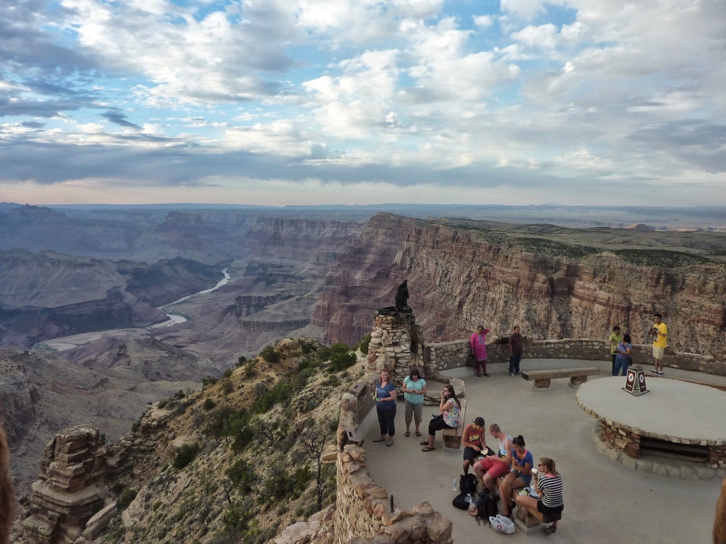
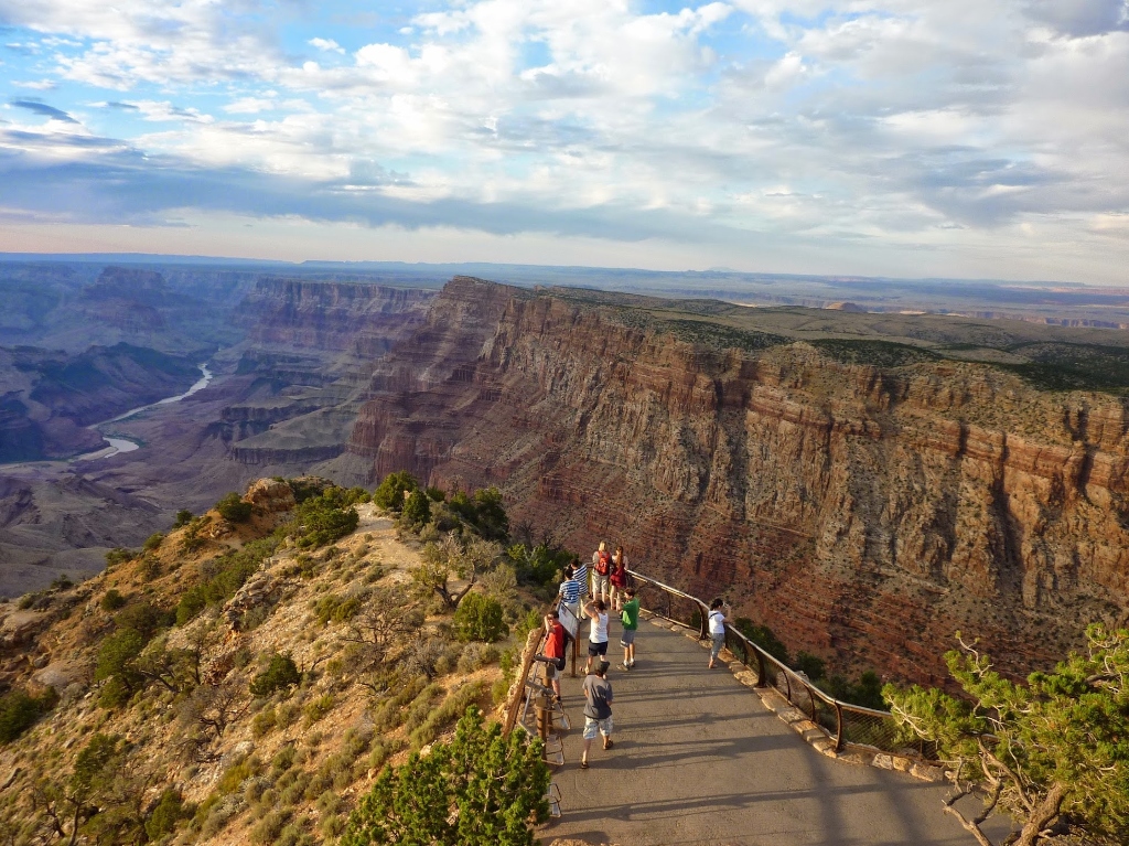
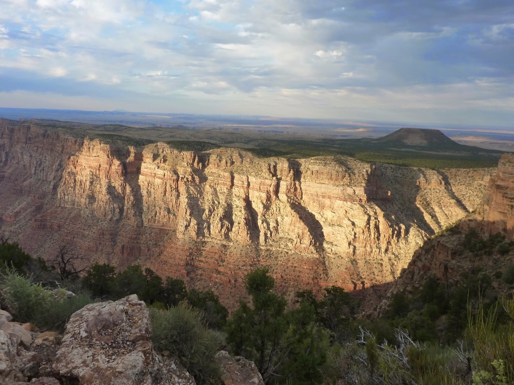
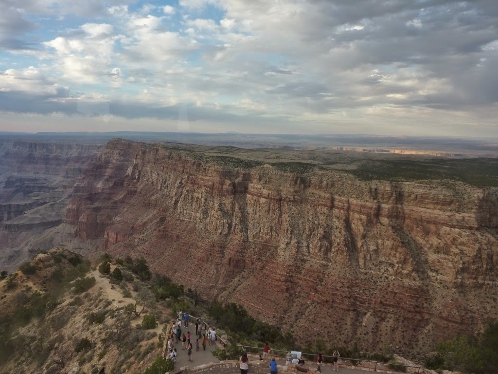
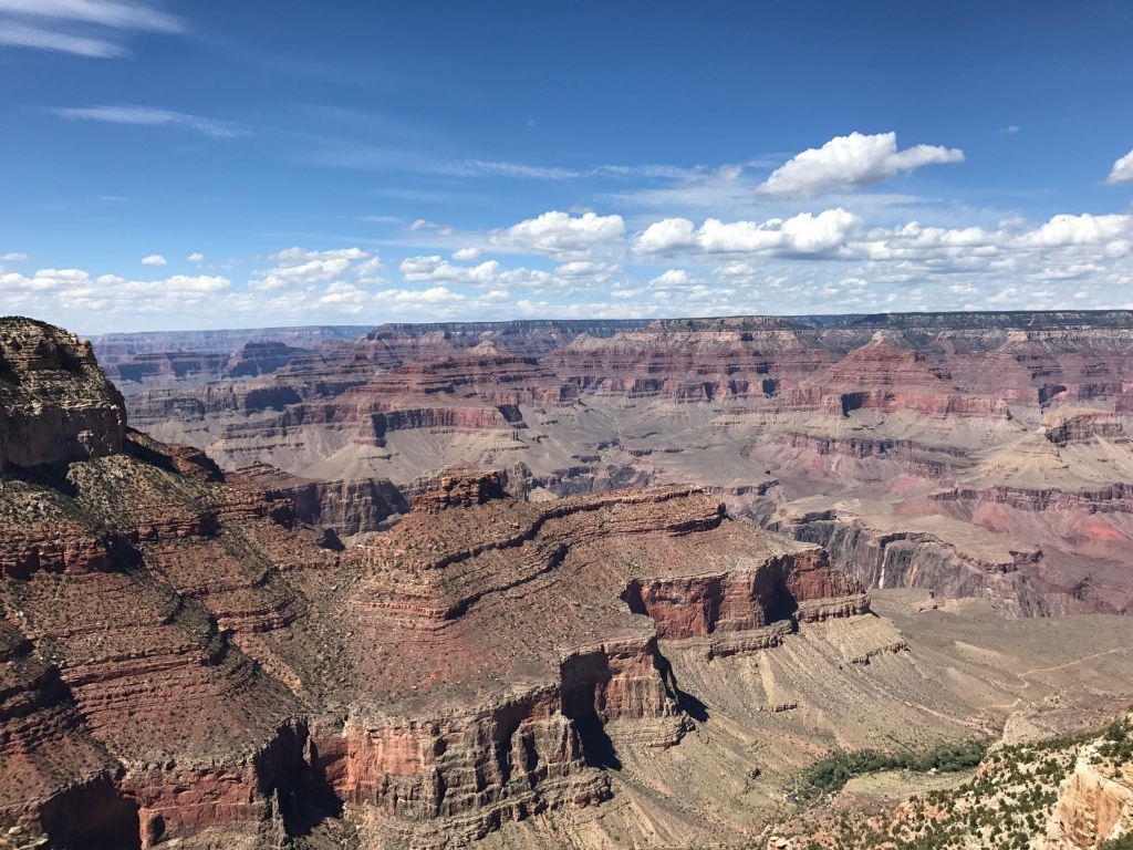
The Grand Canyon is one of the most spectacular geological formations on Earth, and one of the few features visible from low Earth orbit. Carved over millions of years by the Colorado River, the canyon exposes nearly 2 billion years of geological history in its layered rock walls, making it a natural laboratory for understanding Earth's deep past.


Dimensions
446 km long, up to 29 km wide, and over 1,800 m deep. The canyon is so large it creates its own weather patterns.
Geology
Exposes rocks from the Vishnu Basement (1.84 billion years old) to the Kaibab Limestone (270 million years old), with a "Great Unconformity" representing a gap of over 1 billion years.
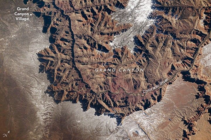
Visible from Space
Astronauts on the ISS regularly photograph the canyon. Its distinct coloration and scale make it identifiable from orbit at ~400 km altitude. SRTM captured its full topography in 2000.
Why We Study It
The canyon is an ideal case study for DEM visualization: extreme elevation variation, dramatic terrain features, and rich data availability in Google Earth Engine.
Brief Geological Timeline
Vishnu Basement Rocks form deep in Earth's crust through volcanic activity and tectonic compression.
Grand Canyon Supergroup deposited: sandstones, shales, and limestones from ancient seas, rivers, and coastal environments.
Paleozoic sedimentary layers begin accumulating: the familiar horizontal strata visible in the canyon walls today (Tapeats Sandstone to Kaibab Limestone).
Laramide Orogeny uplifts the Colorado Plateau, raising it over 2,000 m above sea level and setting the stage for river incision.
The Colorado River begins carving the modern Grand Canyon, cutting through the uplifted plateau at rates of roughly 0.3 mm per year.
NASA's Shuttle Radar Topography Mission (SRTM) maps the canyon's elevation at 30m resolution. This is the dataset we use in today's lab.
Today's Sessions
Load SRTM data, apply color ramps, generate hillshade, and create terrain visualizations in Google Earth Engine.
Lab 15: Visualizing SRTM DataBriefing on synergistic applications of satellite and drone data for sustainability. Introduction to the Drone Image Processing assignment.
Briefing MaterialsStudent-led presentations: each student researches and presents a 5-minute talk on an assigned country's space agency, their EO strategy, and flagship satellites. We have covered NASA and ESA in depth; now it is your turn to teach the class about the rest of the world.
View Assignments BelowSession 3: Lightning Talk Assignments
We have spent this module working extensively with NASA (Landsat, SRTM, MODIS) and ESA (Sentinel, Copernicus). But Earth observation is a global endeavor. Over 70 countries now operate or have operated EO satellites. Your task: become the class expert on one agency and teach us about it.
Presentation Guidelines
Format
5 minutes per student, followed by 2 minutes of class Q&A. You may use slides, a webpage, or simply present from your notes. No formal slide deck required.
What to Cover
- Agency name, country, year founded
- Flagship EO satellite(s) and what they observe
- Data access: is their data free/open?
- One interesting fact or unique capability
Assignments
| Student | Agency / Program | Country | Key Satellites to Research |
|---|---|---|---|
| Aastha Bhatt | ISRO | India | Cartosat, Resourcesat, Oceansat, Chandrayaan |
| Akira Yoshida | JAXA | Japan | ALOS (Daichi), GOSAT, Himawari, EarthCARE |
| Aruna | CNSA / CAST | China | Gaofen series, Fengyun, ZY, Tiangong |
| Assaf Shaked | ISA (Israel Space Agency) | Israel | EROS, Ofek, VENuS (with CNES) |
| David Guevara | AEB / INPE | Brazil | CBERS (with China), Amazonia-1, DETER |
| Ludivine Euranie | CNES | France | SPOT, Pleiades, SWOT, VENuS |
| Nina Velimirovic | Roscosmos | Russia | Resurs-P, Meteor-M, Kanopus-V, Elektro-L |
| Norbert Muzila | AfSA (African Space Agency) | African Union | SANSA (South Africa), NASRDA (Nigeria), EgSA (Egypt) |
| Vanessa Van Decker | CSA | Canada | RADARSAT Constellation, SCISAT, CASSIOPE |
| Venkata Sri Varshini | KASA / KARI | South Korea | KOMPSAT (Arirang) series, Danuri, Nuri |
| Venu Satish | ASI | Italy | COSMO-SkyMed, PRISMA, PLATiNO |
| Vrushali Chittaranjan | NewSpace / CubeSats | Global | Planet (Doves), Spire, ICEYE, Capella |
About AfSA: The African Space Agency
The African Space Agency (AfSA) was established by the African Union in 2023 and is headquartered in Cairo, Egypt. It aims to coordinate the continent's growing space activities, including Earth observation for agriculture, disaster management, and climate monitoring. Several African nations already have national programs: South Africa (SANSA), Nigeria (NASRDA), Egypt (EgSA), Kenya (KSA), Algeria (ASAL), and Ethiopia (ESSTI). AfSA represents a pan-continental approach to space that is unique in the world.
Background: Elevation Data & Terrain Visualization
The SRTM Mission
The Shuttle Radar Topography Mission (SRTM) flew aboard Space Shuttle Endeavour during the STS-99 mission from February 11 to 22, 2000. In just 11 days, it mapped nearly 80% of Earth's land surfaces, creating the first near-global dataset of land elevations.
The payload used interferometric synthetic aperture radar (InSAR): two radar antennas separated by a 60-meter mast extending from the shuttle's cargo bay. By comparing the radar signals received at each antenna (the phase difference), the system computed surface elevation with remarkable precision.
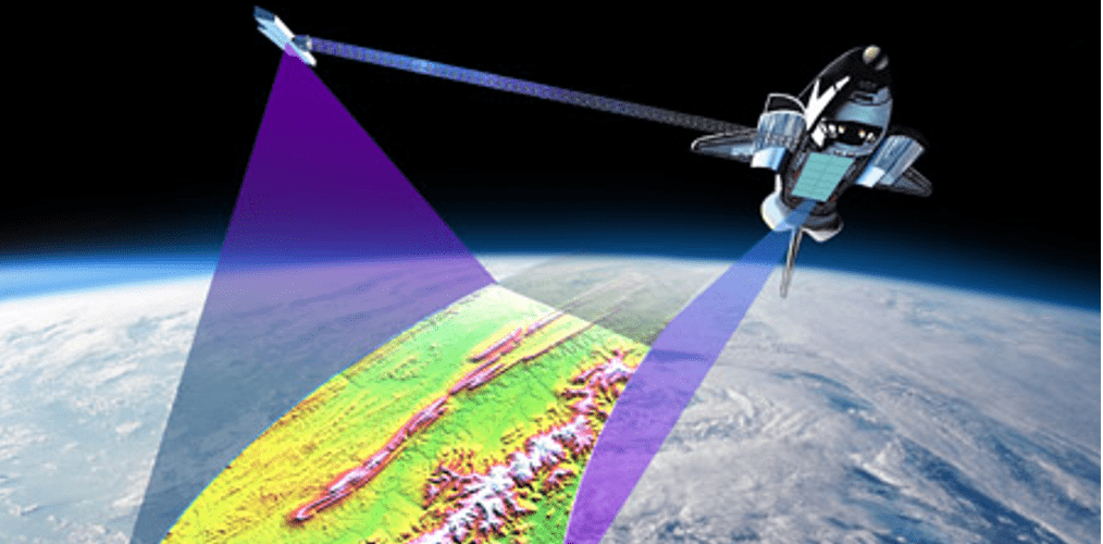
SRTM interferometric radar concept. Two antennas on a 60m mast create stereo radar views to derive elevation. Credit: NASA/JPL-Caltech
Coverage
80% of Earth's land mass, from 60°N to 56°S latitude. 260 orbits over 11 days.
Resolution
~30m (1 arc-second) for the US, ~90m (3 arc-second) globally. Version 3 released 30m worldwide.
GEE Dataset
USGS/SRTMGL1_003 with a single 'elevation' band in meters.
What is a DEM?
A Digital Elevation Model (DEM) is a raster dataset where each pixel stores an elevation value (typically in meters above sea level). Think of it as a grid draped over the Earth's surface, where every cell tells you "how high is this point?" DEMs are the foundation for terrain analysis, hydrological modeling, viewshed calculations, and 3D visualization.
DEM
Digital Elevation Model. Represents the bare earth surface, excluding vegetation and buildings.
DSM
Digital Surface Model. Includes the tops of trees, buildings, and other features. What radar "sees."
DTM
Digital Terrain Model. Similar to DEM but often includes breaklines and morphological features.
What is a Hillshade?
A hillshade is a visualization technique that simulates how sunlight would illuminate terrain from a specific direction and angle. It calculates shadow and light for each pixel based on its slope and aspect (the direction the slope faces), producing a grayscale image that gives a powerful 3D-like appearance to flat maps.
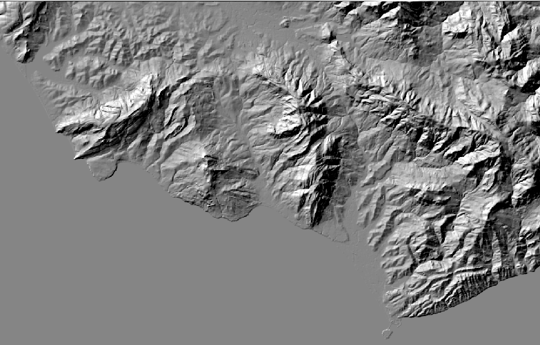
Hillshade rendering of mountainous terrain. Notice how slopes facing the light source (from the northwest) appear bright, while slopes facing away are in shadow, creating a convincing 3D effect from 2D elevation data.
Hillshade Parameters
Azimuth (Light Direction)
The compass direction of the light source in degrees. 270° = light from the west (the conventional default). 0° = north, 90° = east, 180° = south. Changing azimuth reveals different terrain features.
Altitude (Sun Angle)
The angle of the sun above the horizon. 45° is the standard default. Lower angles (e.g., 15°) create longer shadows that highlight subtle features. Higher angles (e.g., 75°) create shorter shadows.
Pro Tip: Combine Hillshade + Color
Professional cartographers overlay a semi-transparent color elevation layer on top of a hillshade to get the best of both worlds: the intuitive color coding of elevation and the 3D terrain perception from shading. In GEE, add the hillshade layer first, then add the color layer with reduced opacity.
Workshop: Lab 15 - Visualizing SRTM Data
- Load DEM data using
ee.Image() - Configure map center and zoom level
- Customize visualization with min/max values
- Apply color palettes to single-band imagery
- Generate hillshade from elevation data
Submit a shareable GEE code URL that includes:
- SRTM data loaded and displayed
- Custom color palette applied
- Hillshade layer created
- Comments explaining your choices
This workshop is graded as part of the T1-B assessment
Color Palettes in Geomorphic Mapping
In terrain visualization, color ramps translate continuous elevation values into intuitive visual representations. The "cold-to-hot" palette is one of the most common approaches in geomorphic mapping, where colors progress from cool tones (low elevation) to warm tones (high elevation), mimicking the natural association between temperature and altitude.
Cold-to-Hot Elevation Palette
Blue (#0000FF)
Low elevation (valleys, river channels, basins). In the Grand Canyon, this represents the canyon floor where the Colorado River flows at ~730m elevation.
Green (#00FF00)
Low-mid elevation (foothills, lower slopes). Often corresponds to riparian zones and vegetated areas in arid environments.
Yellow (#FFFF00)
Mid elevation (plateaus, mesas). The transition zone in the Grand Canyon where inner canyon walls meet the plateau surface.
Orange (#FF8000)
Mid-high elevation (upper slopes, ridgelines). Corresponds to the rim areas and surrounding Kaibab Plateau at ~2,100m.
Red (#FF0000)
High elevation (peaks, summits). In the broader region, this captures the San Francisco Peaks near Flagstaff at ~3,850m.
White (#FFFFFF)
Highest peaks / snow. Mimics the visual appearance of snow-capped summits, reinforcing the elevation-temperature relationship.
Why This Palette Works
The cold-to-hot ramp leverages an intuitive cognitive mapping: we associate blue with water (low), green with vegetation (slopes), yellow-orange with dry terrain (plateaus), red with heat/danger (peaks), and white with snow (summits). This makes elevation data immediately interpretable, even for non-specialists. In GEE, you set this with palette: ['#0000FF', '#00FF00', '#FFFF00', '#FF8000', '#FF0000', '#FFFFFF']
From the Archives: NASA Earth Observatory
A Grand, Snow-Rimmed Canyon
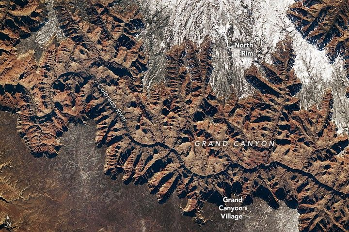
On January 26, 2026, an astronaut aboard the ISS captured photographs of the Grand Canyon after a winter storm dusted the plateau with snow. The South Rim (elevation ~2,100m) and North Rim (~2,400m) were covered in white, while lower, warmer elevations received rain instead. The images demonstrate a phenomenon called relief inversion, where the Sun's position from the south makes the canyon appear like a mountain range rather than a chasm.
The images were acquired with a Nikon Z9 at 400mm focal length during Expedition 74. They highlight the same SRTM terrain we will visualize in today's lab, connecting astronaut photography with remote sensing data.
Read Full NASA Article